Reliability Based Design Optimization
Working Directory and Extraction of necessary files
- Create a working directory in the desired location to keep the LS-OPT project file and input files, as well as the LS-OPT program output, e.g. monte_carlo.
- Extract all the files required for this example from download section into the working directory.
Project Details
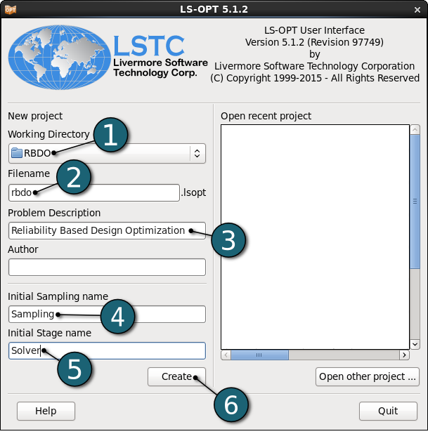
- Select the Working Directory of the LS-OPT project.
- Select a suitable name for the file under Filename (e.g. rbdo. The extension .lsopt is appended by LS-OPT.
- Description of the main task can e.g. be a suitable name for Problem Description ( in this case, Reliability Based Design Optimization, optional) .
- Choose a suitable name under the Initial Sampling name (e.g. Sampling).
- Choose a suitable name under the Initial Stage name (e.g. Solver).
- Click on the Create button to initiate the formation of the input file.
- The main GUI window of LS-OPT opens.
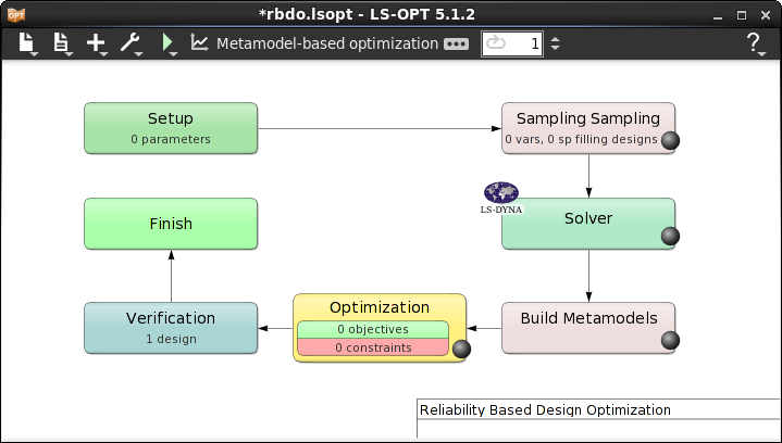
Home Screen Process Flowchart
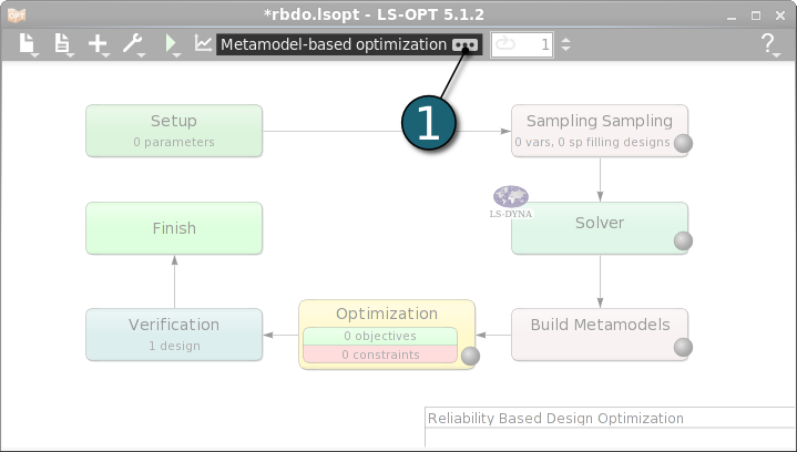
- Click on the Show task settings icon to select the optimization task and strategy.
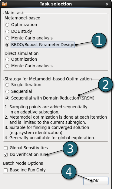
The Task Selection window shall then open.
Define the Main Task
- Select RBDO/Robust Parameter Design for the Metamodel-based main task.
- Select Sequential with Domain Reduction (SRSM) as the Strategy for Metamodel-based Optimization.
- After the last full iteration Do verification run to execute a simulation using the predicted optimal parameter values.
- Click on the OK button to proceed.
- After defining the main optimization task the Home Screen Process Flowchart takes its shape accordingly.
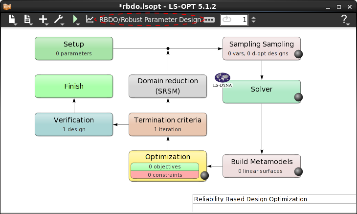
Home Screen Process Flowchart
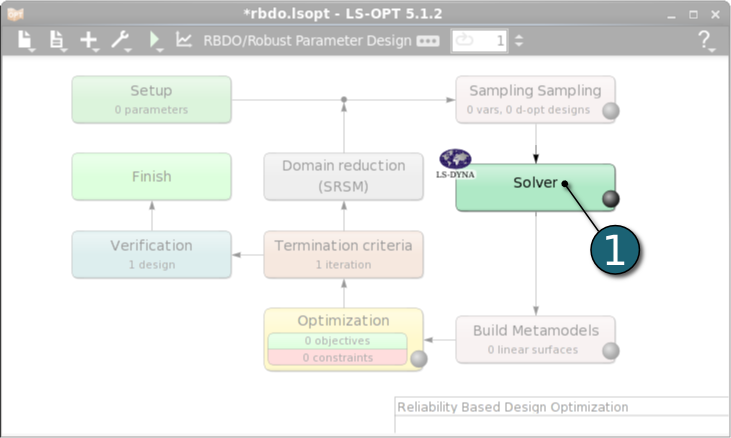
- Double click on the Solver stage.
The Stage Solver dialog shall open.
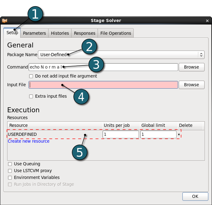
Define Stage Setup
- Select Setup tab.
- Select User-Defined as Package Name.
- For Command type echo N o r m a l which signals LS-OPT a normal termination for the solver stage. Since this is an analytical example, the responses are directly defined directly as expressions depending on the parameter. Note that on Windows a batch script has to be used here.
- For the same reason, no input file is needed in this example. The analytical solution of the problem will simply be defined in the Responses below.
- For efficient usage of the computing power from the machine, choice on handling number of concurrent jobs can be made suitable in this section. For more details see FAQ resources.
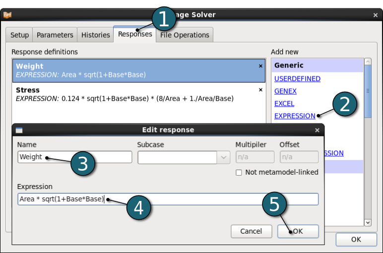
Define Responses
Define Weight
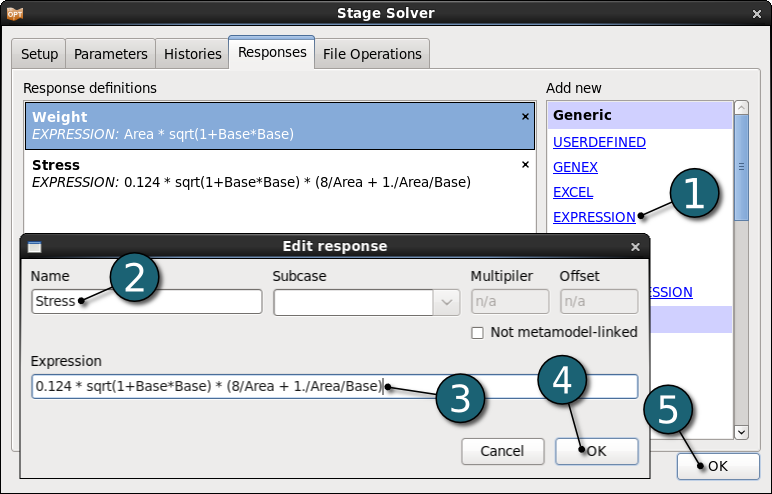
- Select Responses tab.
- Select EXPRESSION as a response type.
- Enter Weight as response Name.
- Enter the Expression
Area * sqrt(1+Base*Base)
to calculate the mass of the structure. - Click on the OK button to finish the definition of the response Weight.
Define Stress
- Select the response type as EXPRESSION.
- Enter Stress as response Name.
- Enter the Expression
0.124 * sqrt(1+Base*Base)
* (8/Area + 1./Area/Base)
to calculate the stress in the structure. - Click on the OK button to end the definition of the response Stress.
- Click on the OK button to proceed.
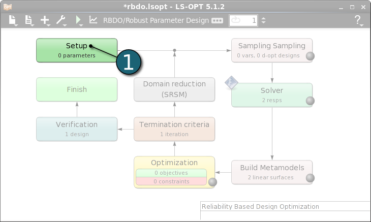
Home Screen Process Flowchart
- Double click on the Setup box to define the design variables.
The Problem globel setup dialog shall open.
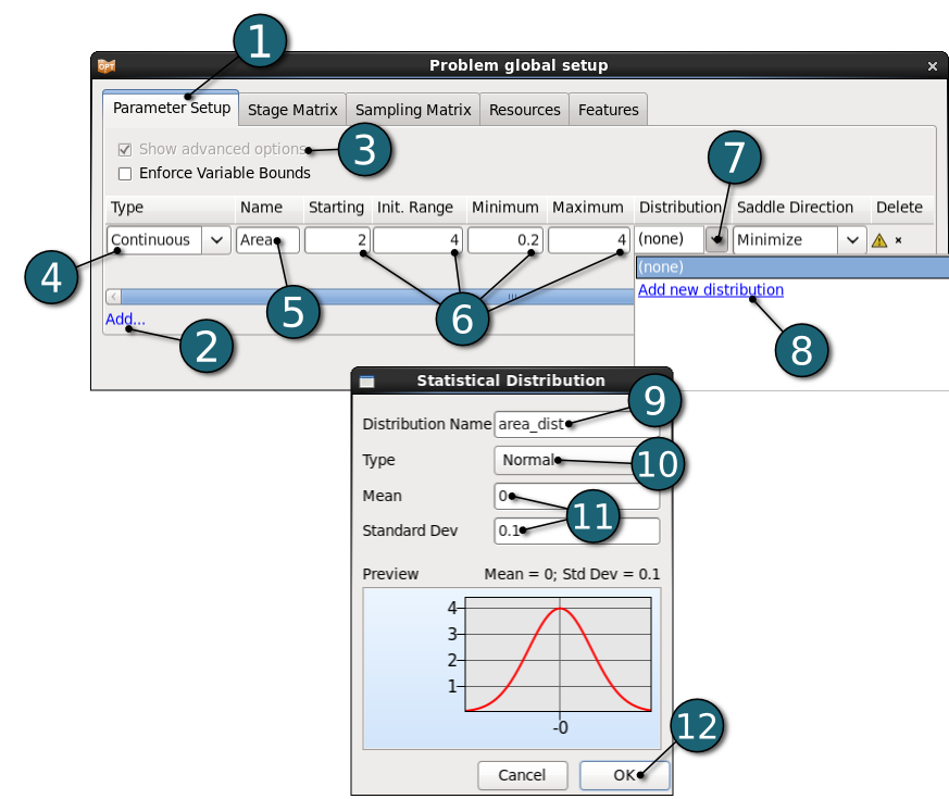
Define Parameters
Define Area
- Select Parameter Setup tab. Since no input file is defined here, the Parameter Setup tab is empty.
- Click on the Add to define new parameter.
- Activate Show advanced options.
- Select the variable Type as Continuous.
- Enter Area for the Name.
- Enter 2, 4, 0.2 and 4 for Starting, Init. Range, Minimum and Maximum, respectively.
- Select the options for Distribution of the variable.
- Click on the Add new distribution.
- Enter area_dist for Distribution Name.
- Select Normal as the Type of distribution.
- Enter 0 and 0.1 for the Mean and Standard deviation, respectively.
- Click on the OK button to define the distribution.
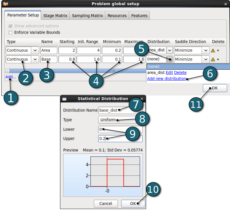
Define Base
- Click on the Add to define new parameter.
- Select the variable Type as Continuous.
- Enter Base for the Name.
- Enter 0.8, 1.6, 0.1 and 1.6 for Starting, Init. Range, Minimum and Maximum, respectively.
- Select the options for Distribution of the variable.
- Click on the Add new distribution.
- Enter base_dist for Distribution Name.
- Select the distribution Type as Uniform.
- Enter 0 and 0.2 for the Mean and Standard deviation, respectively.
- Click on the OK button to define the distribution.
- Click on the OK button to proceed.
Home Screen Process Flowchart
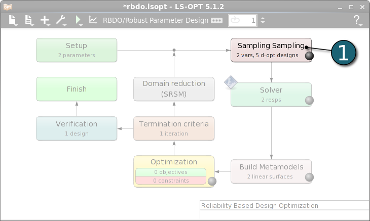
- Double click on the Sampling box in order to define sampling settings.
A Sampling dialog shall open.
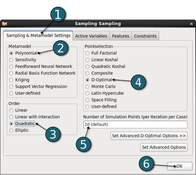
Define Metamodel Settings
- Select Metamodel Settings tab.
- Select the Metamodel type as Polynomial.
- Select the Order of the polynomial metamodel as Quadratic to get more accuracte statistical values.
- Select the Pointselection method as D-Optimal.
- Use the default Number of Simulation Points.
- Click on the OK button to proceed.
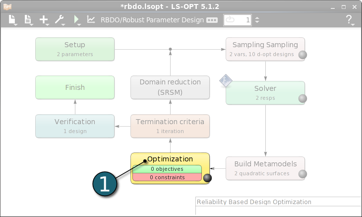
Home Screen Process Flowchart
- Double click on the Optimization box to specify objectives and constraints for the design formulation and the optimization algorithm.
The Optimization dialog shall open.
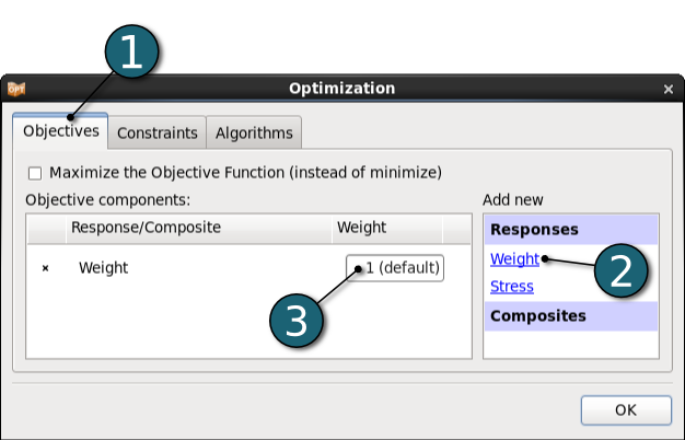
Define Objective
- Select the Objectives tab.
- From Responses list select Weight as the objective.
- Use the default Weight 1. If you have multiple objectives, you may assign different weights to each one according to their importance.
Define Constraints
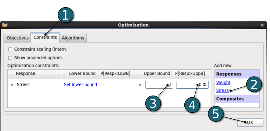
- Select the Constraints tab.
- Select Stress from the Responses list as the optimization constraint.
- Set the Upper Bound as 1.
- For the probability of exceeding the upper bound of the constraint enter 0.05.
- Click on the OK button to proceed.
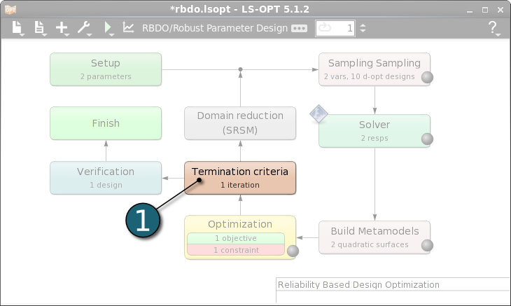
Depending on the optimization task and strategy, the user can specify tolerances on the design change, the objective function change or the accuracy of the metamodel. The user can also specify whether termination is reached if any one, or all of these criteria are met.
Home Screen Process Flowchart
- Double click on the Termination criteria box.
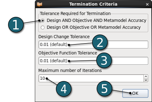
A Termination Criteria window shall open.
Define Termination Criteria
- Select Design AND Objective AND Metamodel Accuracy option for Tolerance Required for Termination.
- Use the default value 0.01 for the Design Change Tolerance.
- Use the default value 0.01 for the Objective Function Tolerance.
- Enter 10 for the Maximum number of iterations.
- Click on the OK button to proceed.
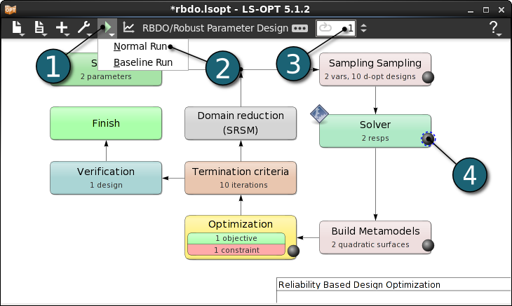
Home Screen Process Flowchart
Run LS-OPT
- Click on the Run button on the Control Bar.
- Click on Normal Run.
- The user can get information on the status of the current iteration during execution.
- For every stage the user has the option to observe the progress of the program execution by selecting the LED at the corner on the Stage box. It is possible to observe the Progress and View Log for more information about the execution process.
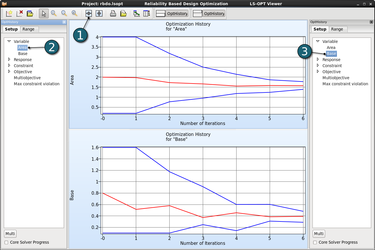
The optimization history of a variable, dependent, response, constraint, objective, multi-objective or the approximation error parameters of pure responses (not composites or expressions) shows the changes of the respective values of the optimum over the iterations.
Home Screen Process Flowchart
- Click on the Open the viewer icon in the control bar on the Home Screen Process Flowchart.
A New Plot window shall open.
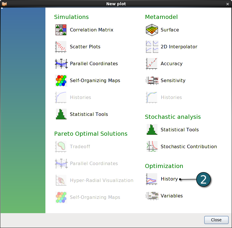
- Choose History under Optimization.

Optimization Histories
- Click on the Split vertical button to display two optimization history plots in the same window, i.e. the history of the variables Area and Base.
- Select variable Area in the Setup dialog.
- Select variable Base in the Setup dialog.
- The red line displays the variable value, and the blue lines the subregion bounds considered for the respective iteration.
Constraint & Objective
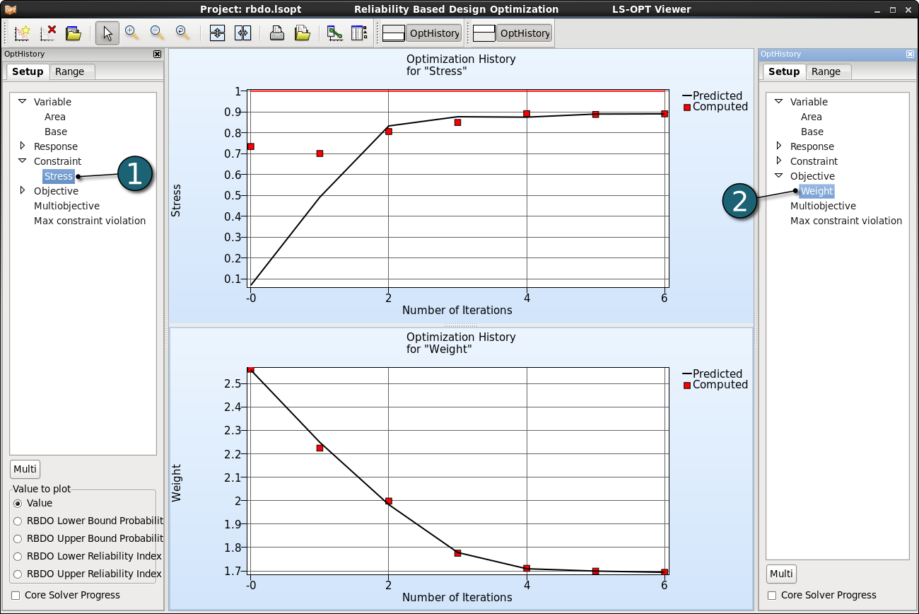
- Select constraint Stress in the Setup dialog.
- Select objective Weight in the Setup dialog.
- In the plot below a black solid line indicates the predicted values for the objective and constraint. The red squares represent the computed values of the optimal point of each iteration.
- For the constraints, the lower and upper bounds are displayed with a blue and red line, respectively.
Contraint & Probability
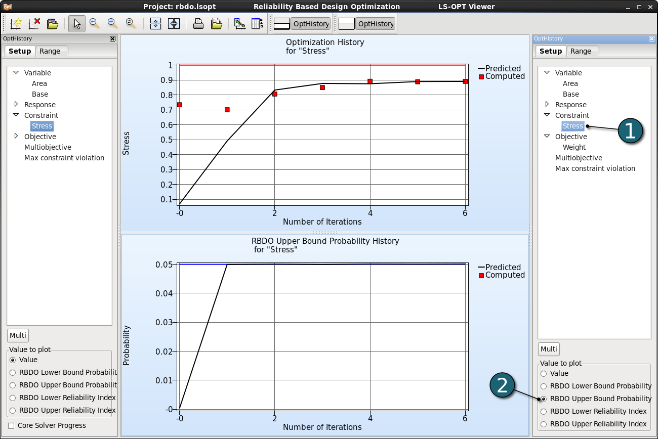
- Select constraint Stress in the Setup dialog of the plot below.
- Select RBDO Upper Bound Probability as the Value to plot.
New Plot - Surface
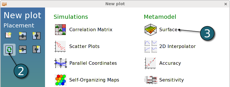
- Click on the New Plot button on the menu bar - ( or click on the View button on the Home Screen Process Flowchart as done in previous step for Optimization Histories).
A New Plot window shall open.
- Select Replace current plot icon.
- Select Surface under Metamodel.

Plot Surface - Settings
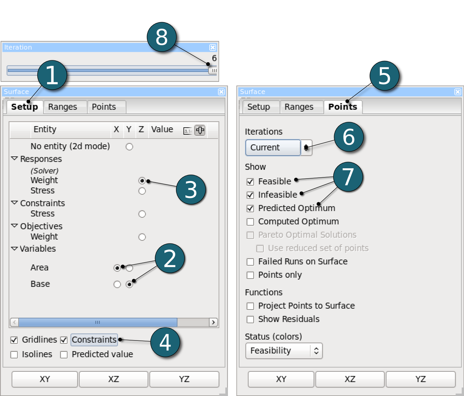
- Select the Setup panel.
- Set the variables Area and Base as x- and y-coordinate, respectively.
- Choose the objective Weight as z-coordinate.
- Display Constraints on the surface.
(Feasible regions are in green, the shade of red shows the degree of infeasibility (number of violated constraints), the colored line show the location where the constraints are exactly met.) - Go to the Points panel.
- Turn Iterations to Current.
- Display the Feasible, Infeasible and Predicted Optimum points.
- Show the surface plot for the last Iteration 6.
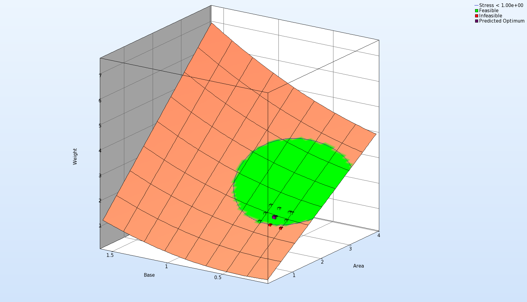
Due to the target failure probability of 0.05, the optimal value is not the lowest value with the feasible region.
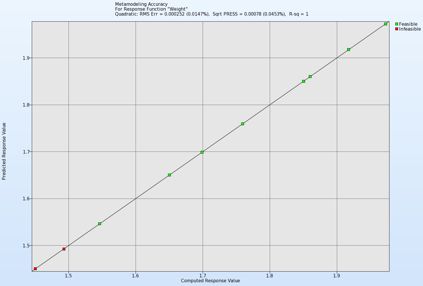
The accuracy of the metamodel fit for the selected response or composite is illustrated in a Predicted vs. Computed plot.
New Plot - Accuracy
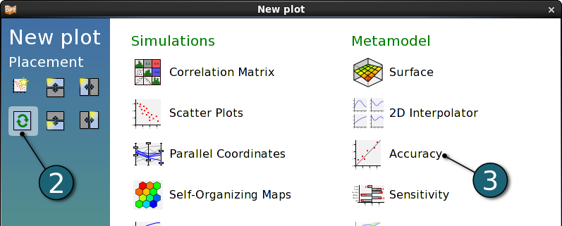
- Click on the New Plot icon in the menu bar - (or click on the Open the viewer icon on the Home Screen Process Flowchart).
A New Plot window shall open.
- Select Replace current plot icon.
- Select Accuracy under Metamodel.

Accuracy Plot Settings
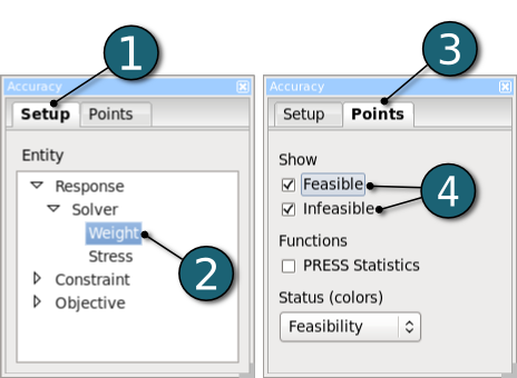
- Select Setup tab.
- Select the objective Weight to display its accuracy.
- Select Points tab.
- Display Feasible and Infeasible points on the accuracy plot.
For Linux : rbdo_linux.tar.gz (1.1 kB)
For Windows : rbdo_windows.zip (1.2 kB)
