Optimizing LS-DYNA input curves
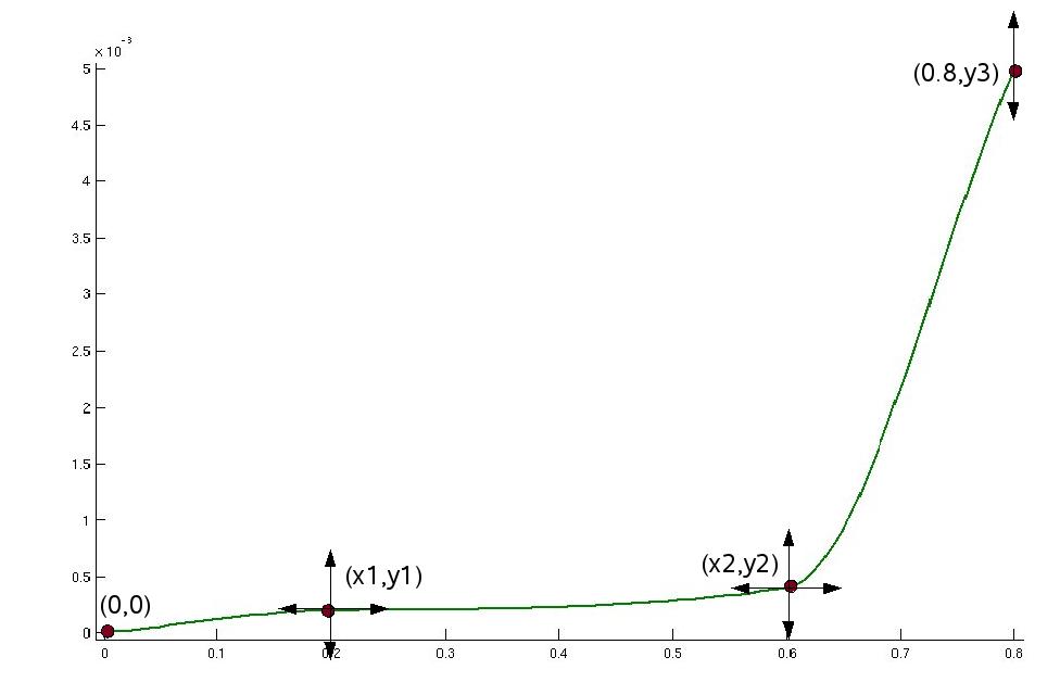
To optimize LS-DYNA input curves, e.g. stress vs. strain data, one solution is to use splines that interpolate a certain number of given points. The coordinates of that points or at least some of them are defined as LS-OPT parameters. Further variables may be defined in the LS-DYNA input file.
Stage 1: Preprocessing
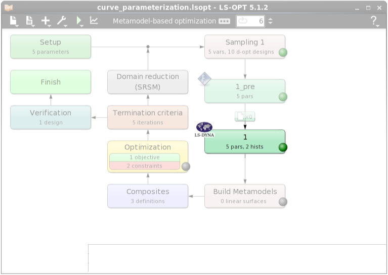
To interpolate the supporting points, the perl program cubic_hermite_interpolation.pl is used as preprocessor in LS-OPT.
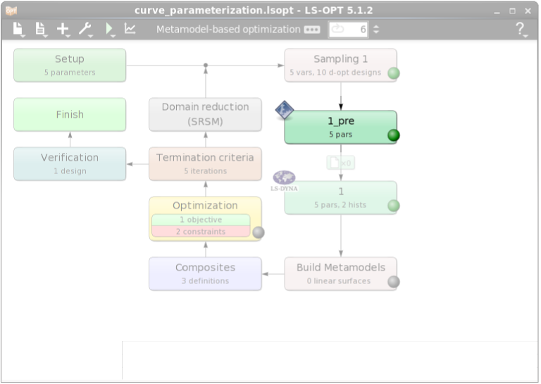
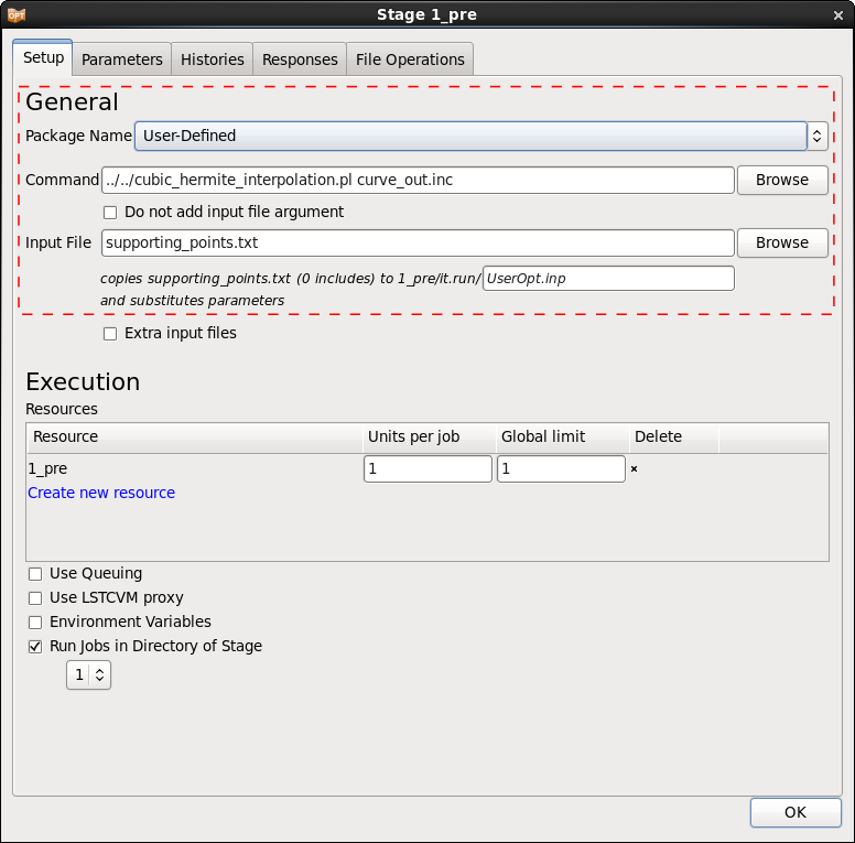
The variables are defined in preprocessor input file supporting_points.txt.
0 0
<<x1>> <<y1>>
<<x2>> <<y2>>
0.8 <<y3>>
Each line contains the coordinates of a supporting point, the number of points is arbitrary and the coordinates may be fixed values and LS-OPT variables, respectively.
Define Composites
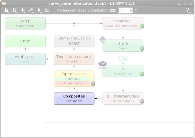
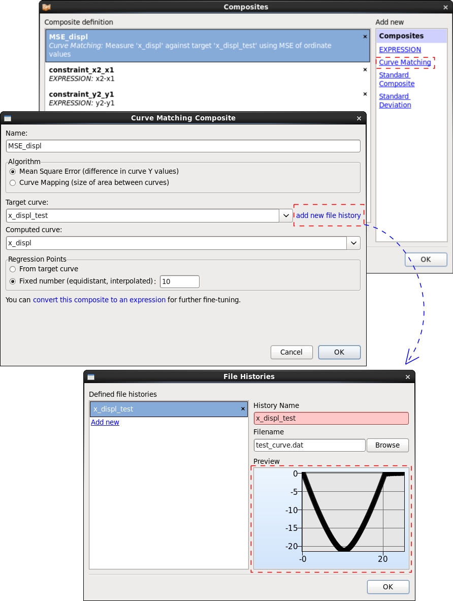
To define an objective we use a Mean Squarred Error composite that compares the displacement test curve test_curve.dat to the computed displacement curves, see http://www.lsoptsupport.com/examples/parameter-identification/history-mse.
Define Objective & Constraints
In the Optimization dialog we can define the objective of the problem.
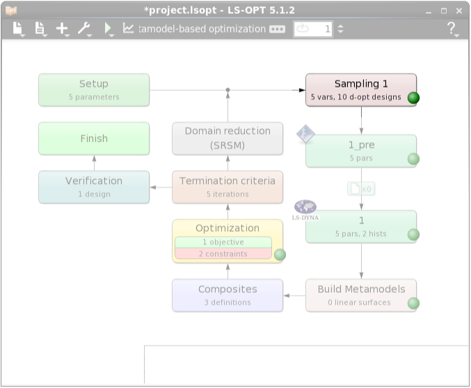
After defining constraints as a sampling constraint in the Sampling dialog we can see them in the Optimization dialog Constraints tab, too.
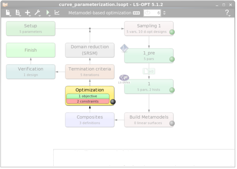
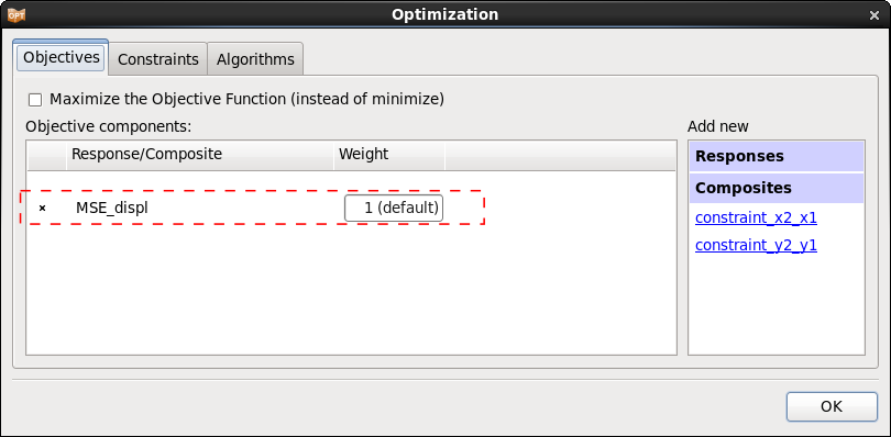
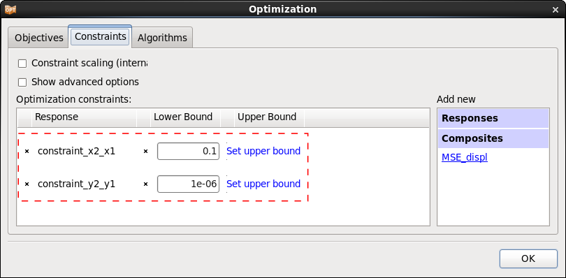
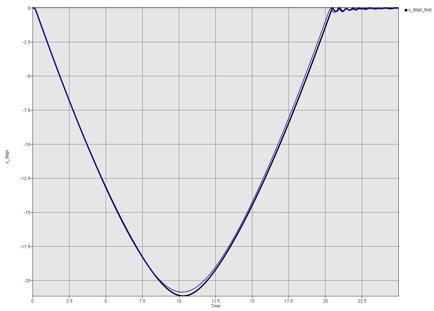
After five iterations, LS-OPT returns a stress vs. strain curve that leads to a displacement curve close to the given test data.
Files
The example files have been prepared for Linux and Windows and are available for download at the end of this document.
Please make sure that the execute permission is set for the Perl program and that the preprocessor and solver commands are adapted to your system.
Stage 2: Processing with LS-DYNA
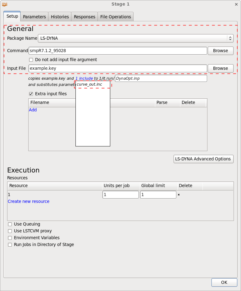
The preprocessing stage with the Perl program returns the file curve_out.inc that contains the output curve in LS-DYNA format and may be used directly as include in the LS-DYNA input file, here in example.key.
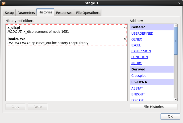
Two histories are defined for this example. x_displ is the displacement curve at node 1651 we want to compare to the given test data. loadcurve is the stress-strain curve generated by the Perl program. This curve is only defined for visualization, it is not used in the optimization.
Define Sampling Constraints
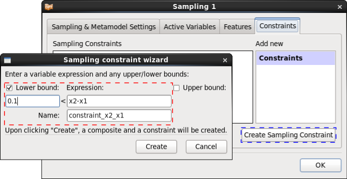
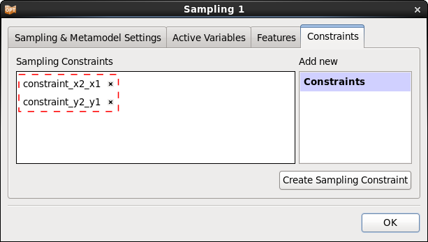
In the case of having constraints on the variables we can define them as sampling constraints in the Sampling dialog.
If we define sampling constraints in the Sampling dialog, these are going to be defined automatically in the Composites and Constraints dialog, too.
In this problem we define the sampling constraints to ensure that the supporting points are monotonically increasing, and hence the stress-strain curve is monotonically increasing.
