Sensitivity Analysis

Responses can depend on many variables, and the computational effort of an optimization strongly depends on the number of variables. In most cases, only a few variables are significant. Sensitivity analysis helps to understand the simulation model and to reduce the design variables used in an optimization. The least significant ones can be de-selected to reduce the computational effort.

Two sensitivity measures are implemented in LS-OPT: Linear ANOVA and GSA/Sobol. Both sensitivity measures are global in nature and are evaluated using the metamodel; hence the metamodel quality is essential to achieve reasonable sensitivity results.

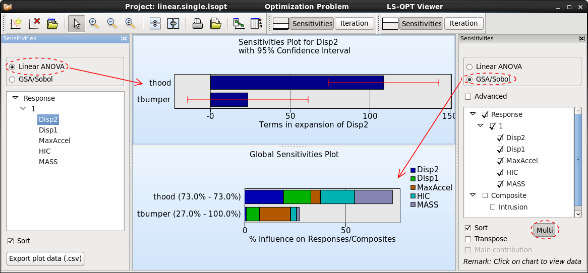
ANOVA is a linear sensitivity measure, whereas GSA/Sobol is non-linear. Therefore, the results are comparable for linear metamodels. ANOVA depicts positive or negative influence, whereas GSA/Sobol just shows the absolute value. An advantage of GSA/Sobol is, that the values are normalized. Hence they can be summed up to determine the influence of a parameter on multiple responses, on a full load case, or on the entire optimization problem.

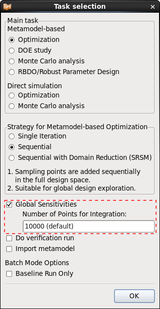
ANOVA is evaluated automatically if metamodels are available, to get GSA/Sobol values, select the Global Sensitivities option in the Task dialog or from the Add menu. To perform a sensitivity analysis, a global metamodel approximation should be used. Two approaches are described in the following.

DOE Task

A global approximation can be achieved by selecting task DOE. To get reasonable results, increase the Number of Simulation Points (per Iteration per Case) at least 2*(n+1), where n is the number of variables. The greater the non-linearity of the response functions, the more points are needed to represent the nonlinearities. Hence the number of points is always a compromise between accuracy and computational effort.

Sequential

An approach for generating a metamodel to a specified prediction accuracy (using the PRESS metric) is to use an iterative method.

Select Metamodel based Optimization for the main task, and the Sequential strategy. Here, the default Number of Points der Iteration can be used, because points are added sequentially. A nonlinear metamodel is recommended, e.g. Radial Basis Functions together with Space Filling point selection sheme.

An appropriate termination criterion for a sequential approach is Response Accuracy Tolerance. Make sure to use the OR option and set the non-accuracy tolerances to 0. The number of iterations to be performed is again a compromise between accuracy and computational effort.

Viewer

Some of the postprocessing options commonly used for sensitivity analysis re as follows:

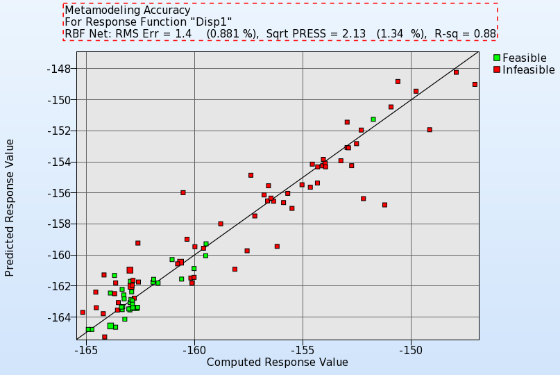
Accuracy

Use the accuracy plot and the error measures displayed in the title to judge the quality of the metamodels.

Sensitivities

The sensitivity measures calculated by LS-OPT, Linear ANOVA and GSA/Sobol can be visualized in the Sensitivities plot. By default, the values are sorted by significance, hence the ranking of the parameters can be directly taken from the order in the plots.

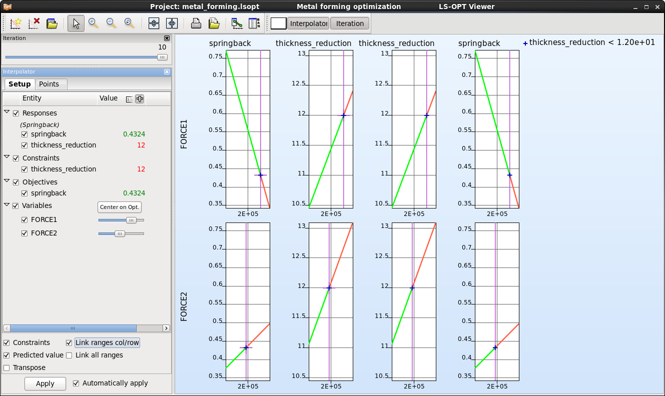
Interpolator

The interpolator plot displays 2D-cross-sections of the metamodels in a matrix for selected responses and variables. Constraints and predicted values for a selected parameter combination can be visualized on the metamodel.