Results
We can plot the response surface of the metamodel we've built. For example, we want to see the effect of the constraint on the optimization solution with respect to the variables thood and tbumper, do it as following:
Home Screen Process Flowchart
- The results can be viewed by selecting the view button on the task bar. A seperate window of LS-OPT Viewer opens up.
LS-OPT Viewer
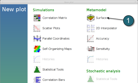
- Select under Metamodel the item Surface.
Constraints
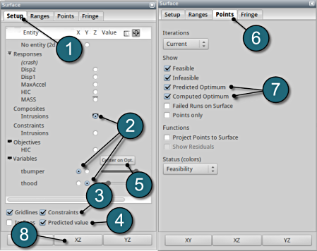
- Select the Setup tab.
- Set the plot coordinates,
- Composites, Intrusions : z-coordinate
- Variables, tbumper : x-coordinate
- Variables, thood : y-coordinate.
- Pick Constraints to visualize feasible and infeasible regions on the metamodel, respectively.
- green : feasible region
- red : infeasible region.
- Choose Predicted value, a cross (+) appears on the surface.
- Click Center on Opt. to locate the cross at the optimal point.
- Select the Points tab.
- Pick Predicted Optimum and Computed Optimum.
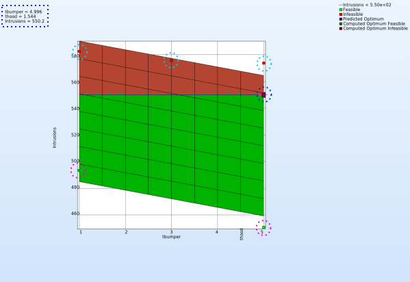
- To view the optimization constraints, we take a 2-D plot of Intrusions vs tbumber (variable).
Plot
- The 2-D plot clearly shows that the points in the red region ( intusions > 550 mm ) form the infeasible solutions, whereas the green points are the feasible solutions.
- The optimum point lies at the periphery of the feasible and infeasible domain. The predicted optimum point values are shown at the top-left corner of the plot.
Objective - HIC Plot
- The primary objective of the optimization is to minmize the HIC.
- Repeat similar steps as the previous plot except for Z-axis select the Objective - HIC.
- Avoid Step. 8, to visulaize in a 3-D plot.
- It is important to note, the optimum is located at the lowest HIC in the feasible region.
- The user has the option to view the various entities by selecting any given point in the plot ( in this case the predicted optimum ). A point selection window opens up.
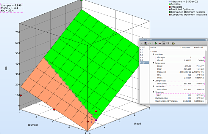
Study the change in each of the variables/responses and the accuracy of the predicted compared to the computed result.
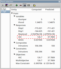
The accuracy of the starting point and the approximate optimum points after the first iteration can be illustrated, e.g. for the response HIC you may find:
New Plot
- To view a new plot select the plot botton on the task bar. A seperate window of LS-OPT Viewer opens up.
LS-OPT Viewer
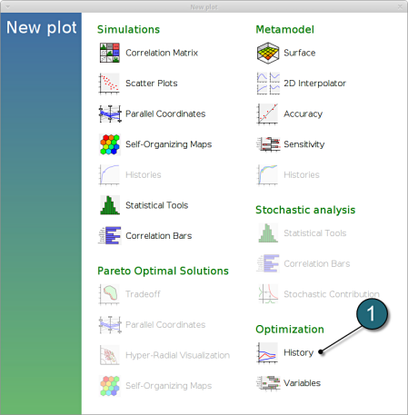
- Select under Optimization the item History.
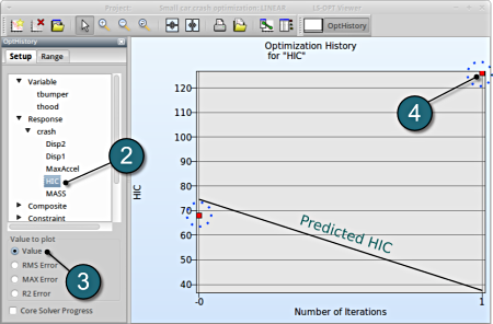
- From the left side of the window select Responses → HIC.
- For Value to Plot select Value.
- If you want to see the accurate values, simply click nearby the red points. There appears a table, which states all the computed and predicted data, e.g. computed HIC vs. predicted HIC.
→ You can find out the appropriate values for the predicted (black) and the computed (red points) results. More iterations may lead to a better predictive capability.
→ A quality analysis is expected when the predicted (black line) and the computed (red points) are in close proximity.
(Note the range of the values when assessing the accuracy)
Predicted results compared to the computed result.
The user can select the respective points and compare the predicted values to the computed results for every iteration :
| Start ( 0.Opt ) | First Iteration ( 1.Opt ) | |||||||||||||||
| Predicted | Computed | Predicted | Computed | |||||||||||||
| thood | 1 | 1.549 | ||||||||||||||
| tbumper | 3 | 5 | ||||||||||||||
| MASS | 0.4103 | 0.4103 | 0.657 | 0.6571 | ||||||||||||
| Intrusion | 577.3 | 575.7 | 550 | 550.4 | ||||||||||||
| HIC | 74.64 | 68.02 | 37.78 | 126.7 | ||||||||||||
| Max. Constr. Violation | 27.28 | 25.69 | 9.919e-5 | 0.3957 | ||||||||||||
What is the approximation error of the result?
The approximation error indicators (predict the metamodel accuracy of the results) can be visualized in the LS-OPT Viewer.
New Plot
- To view a new plot select the plot button on the task bar. A seperate window of LS-OPT Viewer opens up.
LS-OPT Viewer
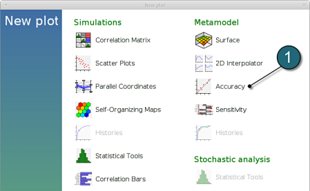
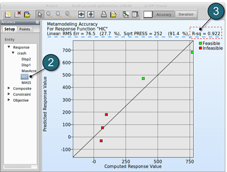
- Select under Metamodel the item Accuracy
- From Entity select Responses → HIC.
- We can find RMS Error and R2 (R-sq) above the plot.
→ Despite the coefficient of determination (R2) being high (=0.922), the RMS Error may need further improvement, e.g. more iterations or selection of a more suitable metamodel (e.g. Feedforward Neural Network or Radial Basis Function Network). Nevertheless for a raw estimate the result may be considered as acceptable.
→ It is important to note that the metamodel performs poor in cross-validation test using the SPRESS method. A relatively high SPRESS value (=91.4%) justifies a low confidence and a low predictive capability of the fitted metamodel.
- With the same procedure you may find the RMS Error, R² and SPRESS Residual of the other responses:
|
|
Mean Response Value |
RMS Error |
R2 |
SPRESS Residual |
|
MASS |
0.7742 |
0 |
1 |
0 (0%) |
|
Disp1 |
-159.3827 |
2.0309 (1.27%) |
0.4783 |
6.68 (4.19%) |
|
Disp2 |
-694.5841 |
5.5486 (0.80%) |
0.9896 |
18.2 (2.62%) |
|
HIC |
275.726 |
76.5620 (27.74%) |
0.9225 |
252.11 (91.43%) |
Which variable appears to be the most important?
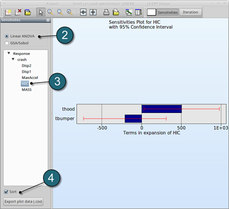
The significance of a variable for a response can be illustrated with ANOVA (analysis of variance) or GSA/Sobol (global sensitivity analysis), e.g for the response HIC you may find:
New Plot
- To view a new plot select the plot button on the task bar. A seperate window of LS-OPT Viewer opens up.
LS-OPT Viewer
ANOVA
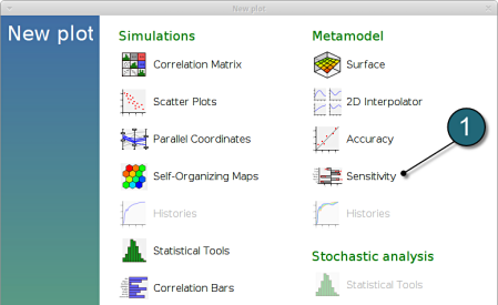
- Select under Metamodel select the item Sensitivity
- Select Linear ANOVA in the new window.
- From Response select HIC.
- Sort the variables according to their significance for HIC.
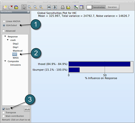
- Select GSA/Sobol.
- From Response select HIC.
- Sort the variables according to their significance for HIC.
→ We come to the same conclusion by using GSA. The influence of thood on HIC is 84.9%, larger than that of tbumper (15.1%).
GSA is a non-linear sensitivity measure, but evaluated on the metamodel, which is linear here. Hence it should lead to the same ranking than ANOVA.

