Robustness of Metal Forming
Working Directory and Extraction of necessary files
- Create a working directory in the desired location to keep the LS-OPT project file and input files, as well as the LS-OPT program output, e.g. monte_carlo.
- Extract all the files required for this example from download section into the working directory.
Project Details
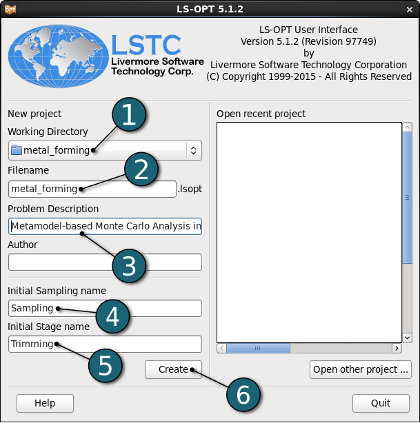
- Select the Working Directory of the LS-OPT project.
- Select a suitable name for the file under Filename (e.g. metal_forming). The extension .lsopt is appended by LS-OPT.
- Description of the main task can e.g. be a suitable name for Problem Description ( in this case, Metamodel-based Monte Carlo Analysis in Metal Forming, optional).
- Choose a suitable name under the Initial Sampling name (e.g. Sampling).
- Choose a suitable name under the Initial Stage name (e.g. Trimming).
- Click on the Create button to initiate the formation of the input file.
- The main GUI window of LS-OPT opens.
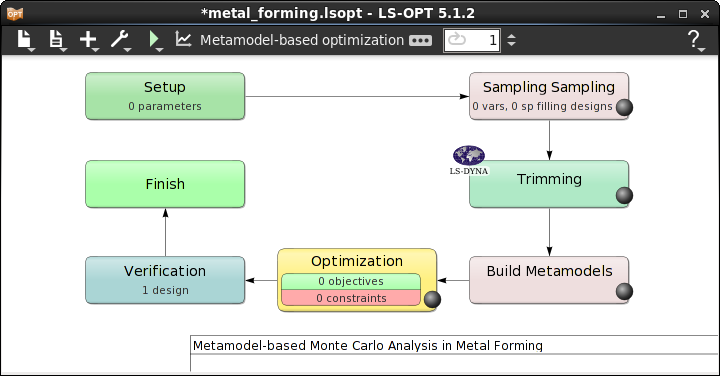
Home Screen Process Flowchart
- Click on the Show task settings icon to select the optimization task and strategy.
The Task Selection window shall then open.
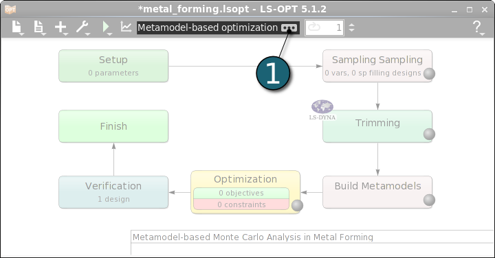
Define the Main Task
- Select Metamodel-based Monte Carlo analysis. In this case, a direct Monte Carlo analysis would require more simulation runs.
- Click on the OK button to proceed.
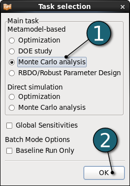
- After defining the main task the Home Screen Process Flowchart displays the process.
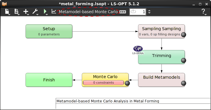
Home Screen Process Flowchart
- Double click on the Trimming box to define the solver step in the simulation process.
The Stage dialog window shall open.
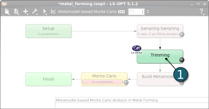
Define Stage Setup for Forming
- Select the Setup tab.
- Select the Package Name LS-DYNA.
- For Command enter smpR7.1.2_95028 (or the respective command available on your system). On Windows, the command has to be specified using the absolute path.
- For Input File browse the LS-DYNA keyword file sheet_metal_forming_trimming.key. Parameters are defined in this file using *PARAMETER keyword. LS-OPT parses this LS-DYNA keyword automatically for parameters and includes.
- Provide trim.igs as an Extra Input File to be copied in the run directories.
- For efficient usage of the computing power from the machine, choice on handling number of concurrent jobs can be made suitable in this section. For more details see FAQ resources.
- Click on the OK button to proceed.
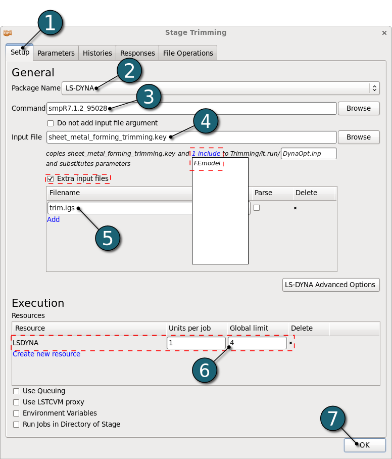
Home Screen Process Flowchart
Add Stage
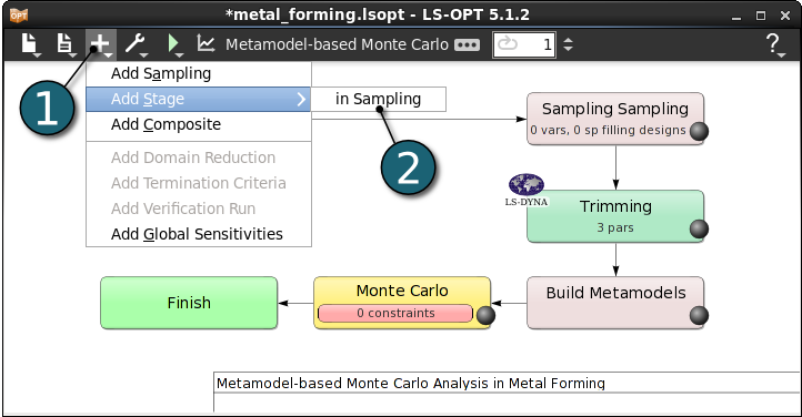
- Click on the Add menu in the control bar.
- Select Add Stage --> in Sampling Sampling for the second step Trimming in the metal forming process.
Enter Simulation as the Name for new stage.
Dependencies of Stages
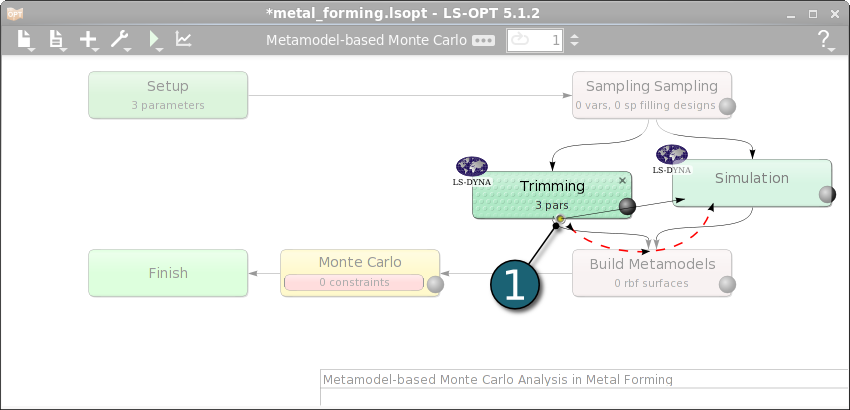
- The dependency of the stages is set by dragging the arrow head from the stage Trimming to the stage Simulation.
- After connecting the two stages to each other we can re-position the stage Trimming for the sake of nice view of flowchart by dragging with simple left-mouse click, or use the Re-layout Stages option from the Tools menu.
File Transfers
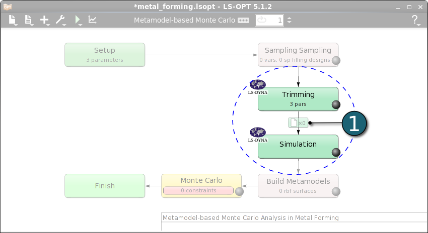
- Since the stage Simulation uses the output file of the stage Trimming as an include file (dynain), the definition of a file transfer is necessary. Click on the File Transfers icon between the two stages. Another option to make the files available for the Trimming stage is to use the Run in directroy of stage option in the Stage dialog Setup tab.
The File Transfers dialog will open.
- Click on Add option to define a file transfer.
- Select the file transfer Operation as Copy.
- Enter the filename of the Source File as dynain.
- Enter the name of the Destination File as dynain.
- In case the operations fails (on Error) select the operation to be applied as fail. The job will return an error termination and LS-OPT won't run the downstream stages for this sampling point.
- Click on the OK button to proceed.

Define Solver Setup for Simulation
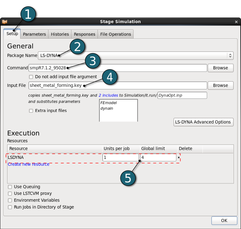
- Open the Simulation - Stage dialog as done for the previous Stage - Forming by double clicking on it. Then select the Setup tab.
- Select the Package Name LS-DYNA.
- For Command enter smpR7.1.2_95028 (or the respective command available on your system). On Windows, the command has to be specified using the absolute path.
- For Input File browse the LS-DYNA keyword file sheet_metal_forming.key.
- For efficient usage of the computing power from the machine, choice on handling number of concurrent jobs can be made suitable in this section. For more details see FAQ resources.
Define Responses
Define FLD_upper_surface
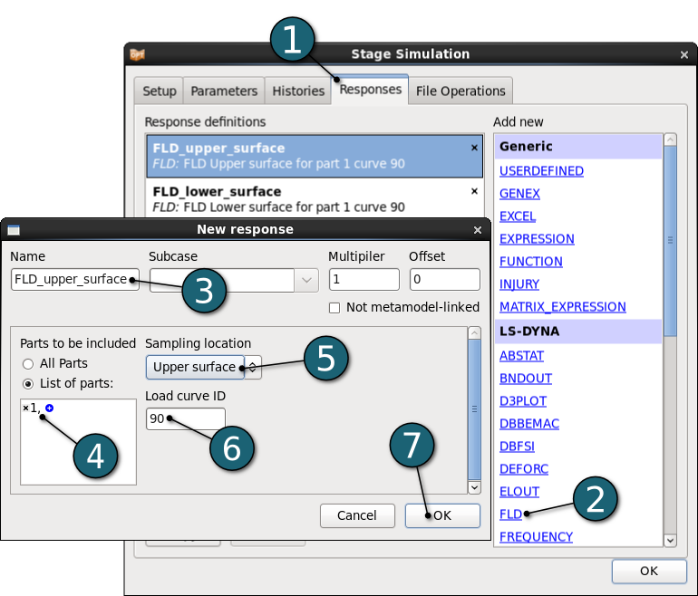
- Select the Responses tab in Stage dialog.
- Select the response as the LS-DYNA d3plot result FLD (Forming Limit Diagram) on the right side of the stage dialog among the response types list.
- Enter the response Name as FLD_upper_surface.
- Enter the List of Parts to be included as 1.
- Select Sampling location as Upper surface.
- Enter the Load curve ID as 90.
- Click on the OK button to end the response definition.
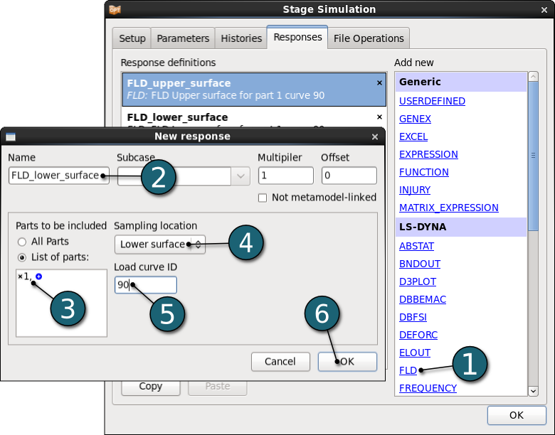
Define FLD_lower_surface
- Select the response as the LS-DYNA d3plot result FLD (Forming Limit Diagram) on the right side of the stage dialog among the response types list.
- Enter the response Name as FLD_lower_surface.
- Enter the List of Parts to be included as 1.
- Select Sampling location as Upper surface.
- Enter the Load curve ID as 90.
- Click on the OK button to end the response definition.
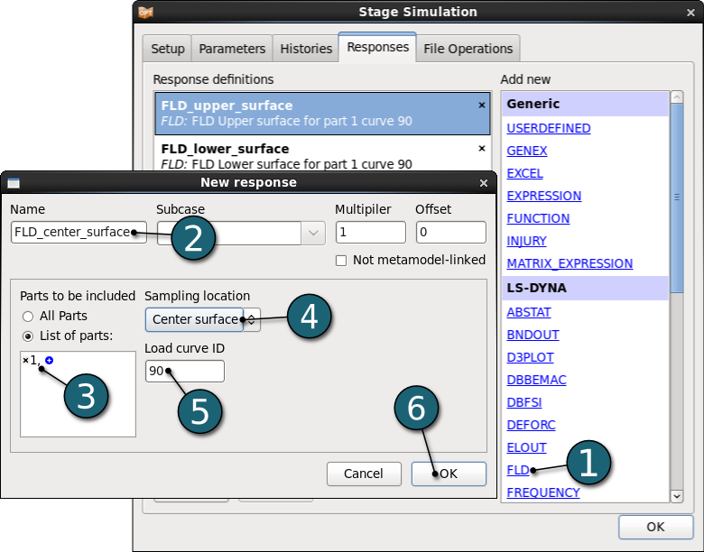
Define FLD_center_surface
- Select the response as the LS-DYNA d3plot result FLD (Forming Limit Diagram) on the right side of the stage dialog among the response types list.
- Enter the response Name as FLD_center_surface.
- Enter the List of Parts to be included as 1.
- Select Sampling location as Upper surface.
- Enter the Load curve ID as 90.
- Click on the OK button to end the response definition.
Define THICKNESS
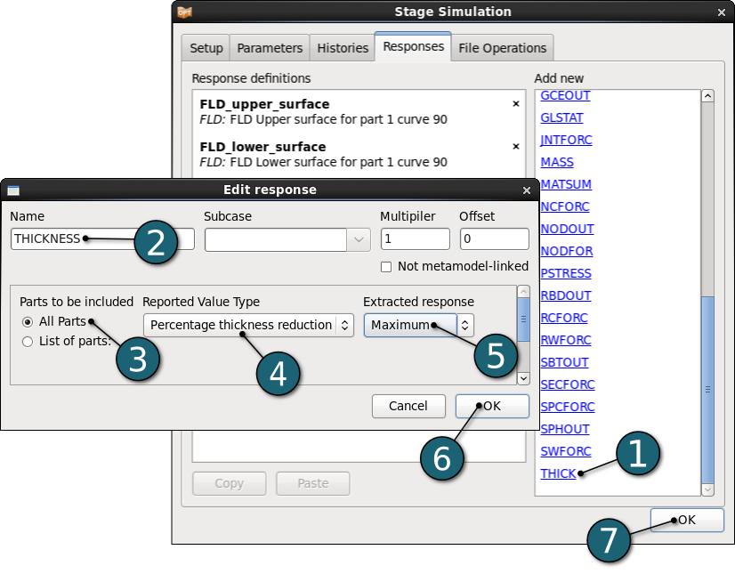
- Select the response as the LS-DYNA d3plot result THICK on the right side of the stage dialog among the response type list.
- Enter the name as THICKNESS.
- Select All Parts to be included.
- Select the Reported Value Type as Percentage thickness reduction.
- Select the Maximum for the Extracted response.
- Click on the OK button to end the response definition.
- Click on the OK button to proceed.
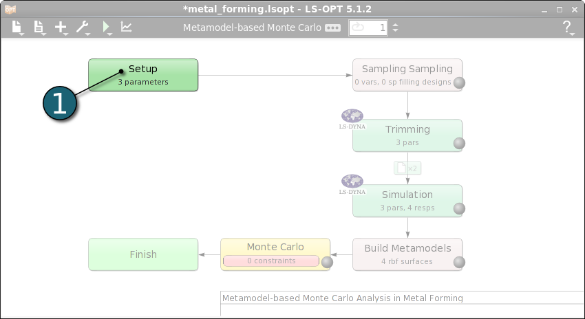
Home Screen Process Flowchart
- Double click on the Setup box for the conversion of parameters to design variables of different types.
The Problem global setup dialog shall open.
Define Parameters
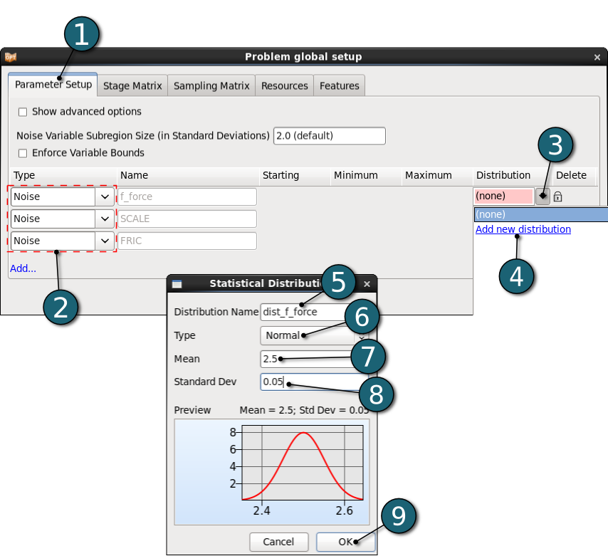
- Select Parameter Setup tab.
- Select the Type for all probabilistic design variables as Noise.
Distribution for f_force
- Open the Distribution settings dialog to define the distribution of variable f_force.
- Click on Add new distribution.
- Enter dist_f_force as the Distribution Name.
- Select the distribution Type as Normal.
- Enter 2.5 for Mean value.
- Enter 0.05 for Standard Deviation.
- Click on the OK button to end the distribution definition for variable f_force.
Distribution for SCALE
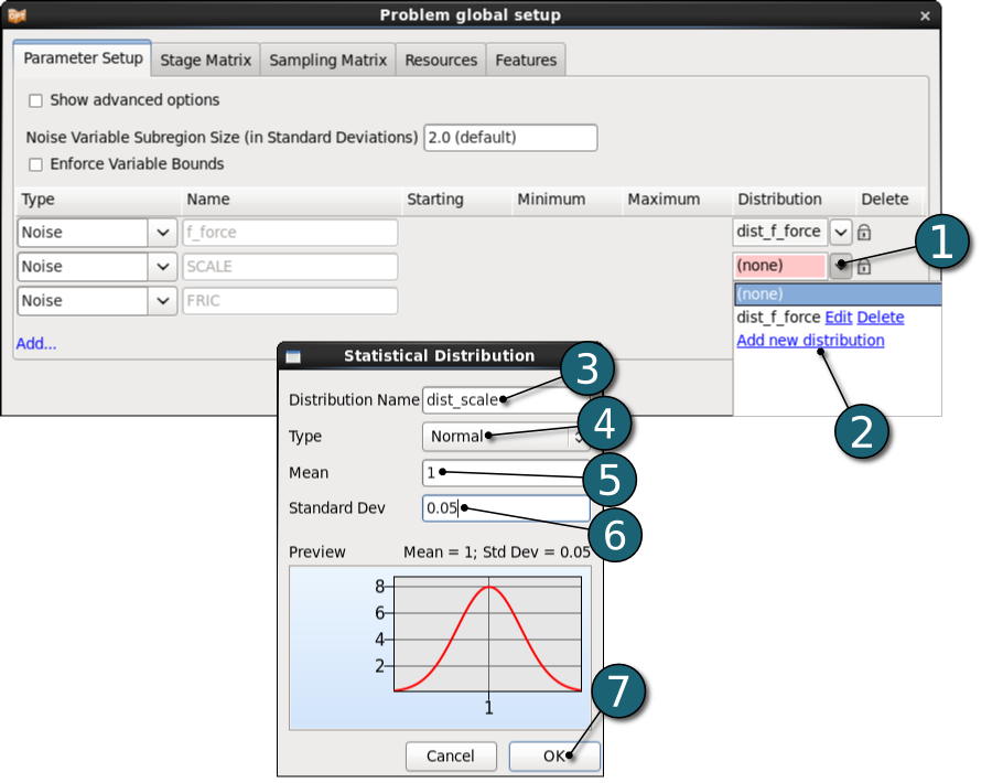
- Open the Distribution settings dialog to define the distribution of variable SCALE.
- Click on Add new distribution.
- Enter dist_scale as the Distribution Name.
- Select the distribution Type as Normal.
- Enter 1 for Mean value.
- Enter 0.05 for Standard Deviation.
- Click on the OK button to end the distribution definition for variable SCALE.
Distribution for FRIC
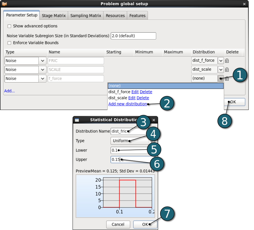
- Open the Distribution settings dialog to define the distribution of variable FRIC.
- Click on Add new distribution.
- Enter dist_fric as the Distribution Name.
- Select the distribution Type as Uniform.
- Enter 0.1 for Lower value.
- Enter 0.15 for Upper value.
- Click on the OK button to end the distribution definition for variable FRIC.
- Click on the OK button to proceed.
Home Screen Process Flowchart
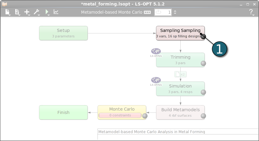
- Double click on the Sampling box in order to define sampling settings.
A Sampling dialog shall open.
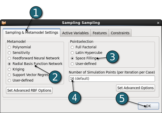
Define Metamodel Settings
- Select Metamodel Settings tab.
- Select Radial Basis Function Network as Metamodel type. All statistics will be evaluated on the metamodel, hence we need a good global metamodel.
- Select Space Filling as Pointselection method.
- Enter 16 as default for the Number of Simulation Points.
- Click on the OK button to proceed.
Home Screen Process Flowchart
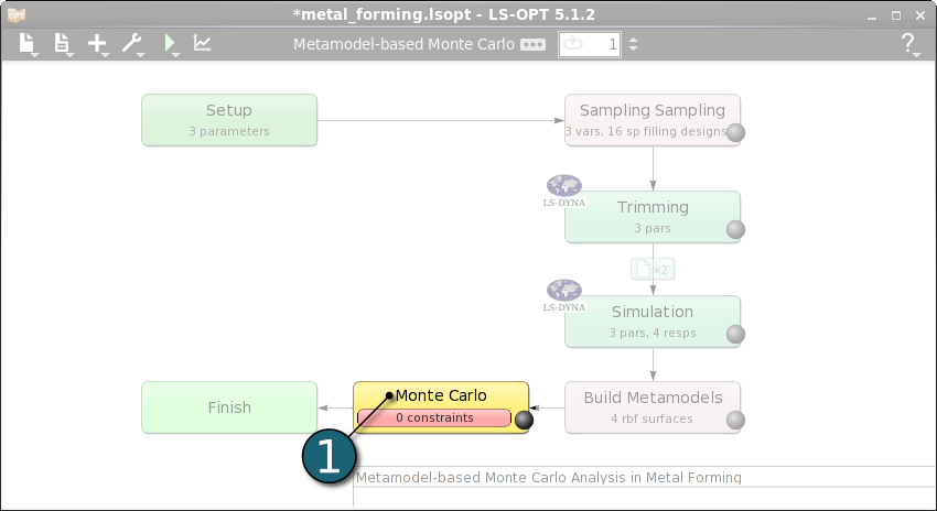
- Double click on the Monte Carlo box.
The Optimization dialog shall open.
A Monte Carlo Analysis does not use objective functions since no optimization is performed, but constraints may be defined to evaluate the probability of failure.
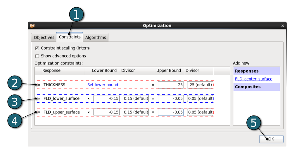
Define Constraints
- Select Constraints tab.
- Select the response THICKNESS to be constrained with the Upper Bound of 25.
- Select the response FLD_lower_surface to be constrained with the Lower Bound of -0.15 and the Upper Bound of -0.05.
- Select the response FLD_upper_surface to be constrained with the Lower Bound of -0.15 and the Upper Bound of -0.05.
- Click on the OK button to proceed.
Home Screen Process Flowchart
Run LS-OPT
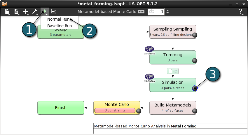
- Click on the Run button on the Control Bar.
- Click on the Normal Run.
- For every stage the user has the option to observe the progress of the program execution by selecting the LED at the corner on the Stage box. It is possible to observe the Progress and View Log for more information about the execution process.
Home Screen Process Flowchart
- Click on the Open the viewer icon in the contral bar on the Home Screen Process Flowchart window.
A New Plot window shall open.
- Choose Surface under Metamodel.


Surface Plot Settings
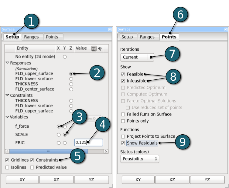
- Select the Setup tab.
- Select the response FLD_upper_surface for the z-axis of the plot.
- Select two of the design variables, e.g. f_force and SCALE, for the x- and y-axis, respectively.
- Set the third design variable, e.g. FRIC, to an arbitrary value. In this case we set FRIC to its mean value, 0.125.
- Display the Constraints on the plot.
- Select Points tab.
- Select the Current Iteration to be displayed on the plot.
- Show the Feasible and Infeasible points on the plot.
- Activate Show Residuals to put forward an idea about the quality of the metamodel.
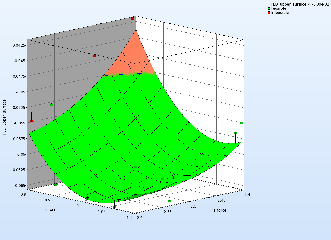
- To display the surface plot of the response FLD_lower_surface select this response in step 2:
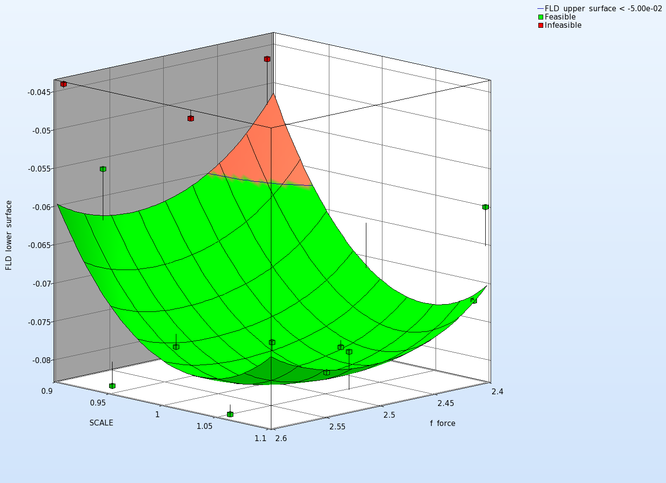
- To display the surface plot of the response THICKNESS select this response in step 2:
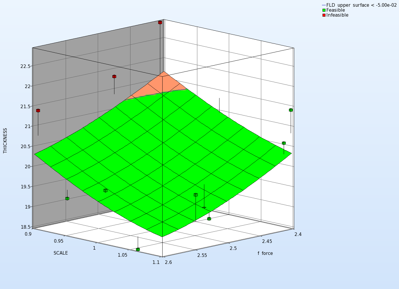
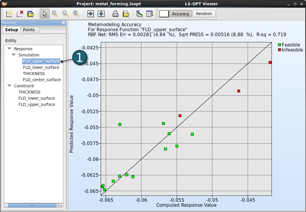
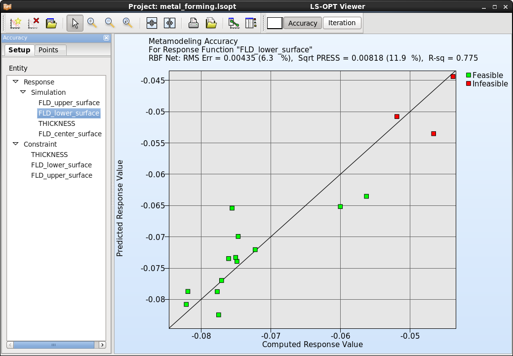
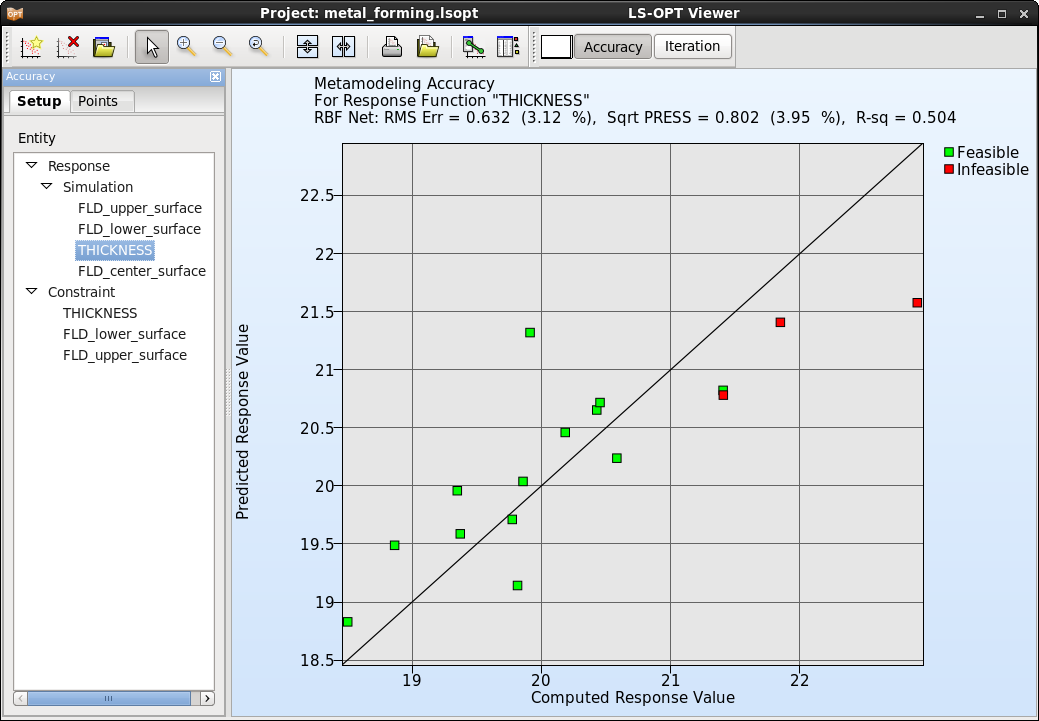
The accuracy of the metamodel fit for the selected response or composite is illustrated in a Predicted vs. Computed plot.
New Plot - Accuracy
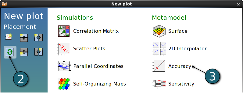
- Click on the New Plot icon in the menu bar - (or click on the Open the viewer icon on the Home Screen Process Flowchart).
A New Plot window shall open.
- Select Replace current plot icon.
- Select Accuracy under Metamodel.

Accuracy Plot Settings
- Select the Response FLD_upper_surface to displays the accuracy of the metamodel for this response in the Setup tab.
- To display the accuracy of the response FLD_lower_surface select FLD_lower_surface in previous step 1:
- To display the accuracy of the response THICKNESS select THICKNESS in previous step 1:
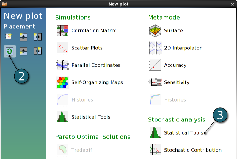
New Plot - Statisctical Tools
- Click on the New Plot icon in the menu bar - (or click on the Open the viewer icon on the Home Screen Process Flowchart).
A New Plot window shall open.
- Select Replace current plot icon.
- Select Statistical Tools under Stochastic analysis.

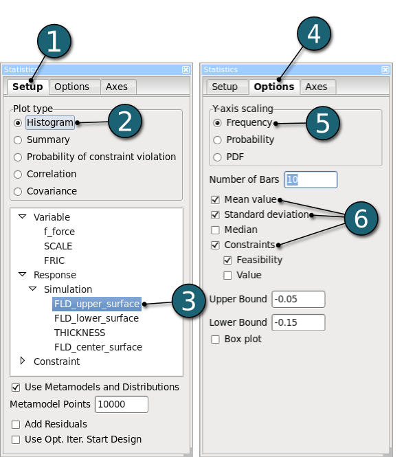
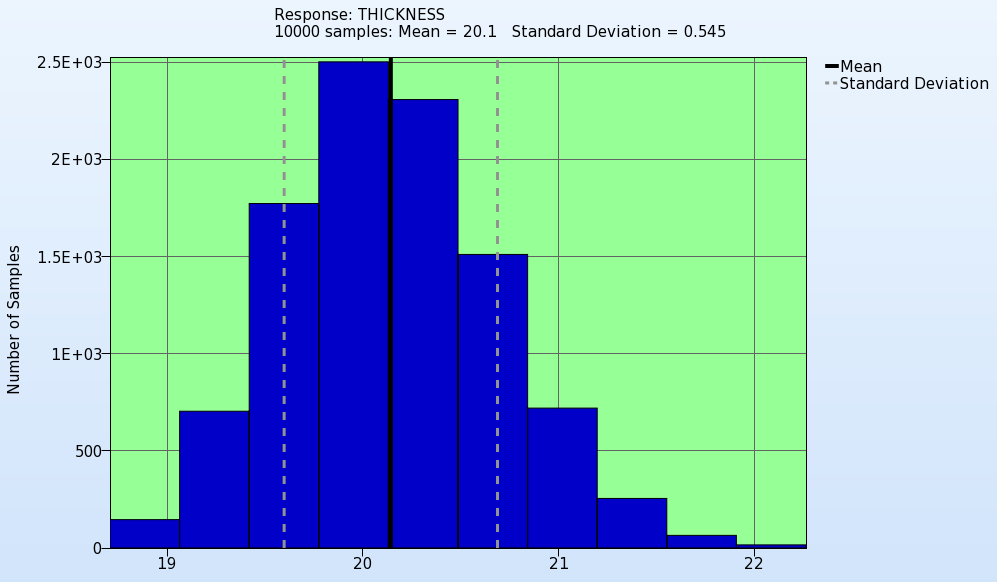
Histogram
- Select Setup tab in the new opened Statictical Tools plot window.
- Select the Plot type as Histogram.
- Select the response FLD_upper_surface to plot its histogram.
- Select Options tab.
- Select Frequency as Y-axis scaling.
- Display Mean Value, Standard deviation and Contraints with Feasibility on the histogram.
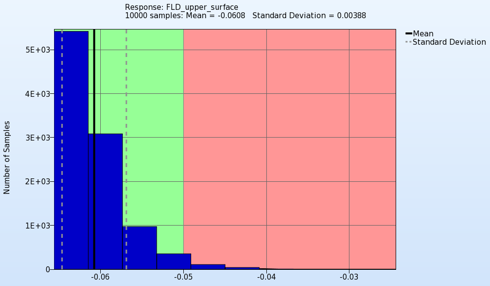
- For the Histogram of the response FLD_lower_surface select this response in step 3:
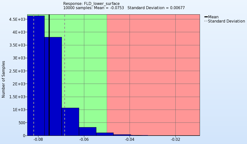
- For the Histogram of the response FLD_lower_surface select this response in step 3:
Probability of constraint violation
- Select Probability of constraint violation as a Plot type.
- Select the Multi option to display more than one Probability of constraints violations.
- Select the three responses FLD_upper_surface, FLD_lower_surface and THICKNESS.
- The 95% confidence interval is shown in red.
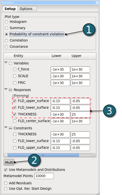

The model is robust, since the probability of failure values are quite small.
New Plot - Stochastic Contribution
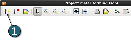
- Click on the New Plot icon in the menu bar - (or click on the Open the viewer icon on the Home Screen Process Flowchart).
A New Plot window shall open.
- Select Replace current plot icon.
- Select Stochastic Contribution under Stochastic analysis.
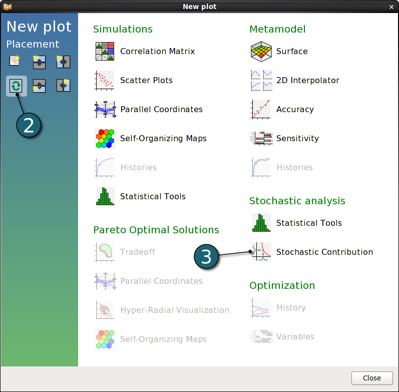
Stochastic Contribution Settings
- Select the Response FLD_upper_surface to display the stochastic contributions of the design variables on this response in the Setup tab.
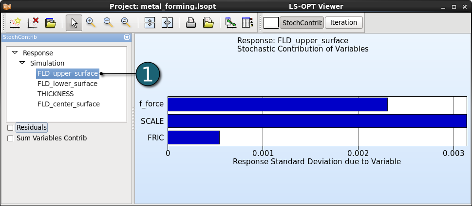
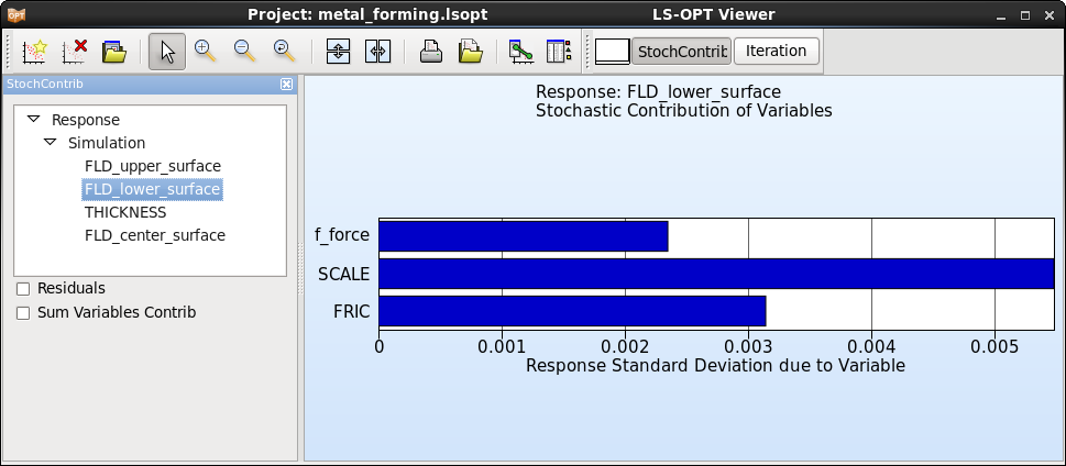
- Select the Response FLD_lower_surface to display the stochastic contributions of the design variables on this response by selecting it in step 1:
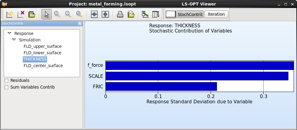
- Select the Response THICKNESS to display the stochastic contributions of the design variables on this response by selecting it in step 1:
For Linux : robustness_metal_forming.tar.gz (134.9 kB)
For Windows : robustness_metal_forming.zip (133.8 kB)
