Metamodel-based MC

 Working Directory and Extraction of necessary files

• Create a working directory in the desired location to keep the LS-OPT project file and input files, as well as the LS-OPT program output, e.g. monte_carlo.
  
• Extract all the files required for this example from download section into the working directory.

Project Details

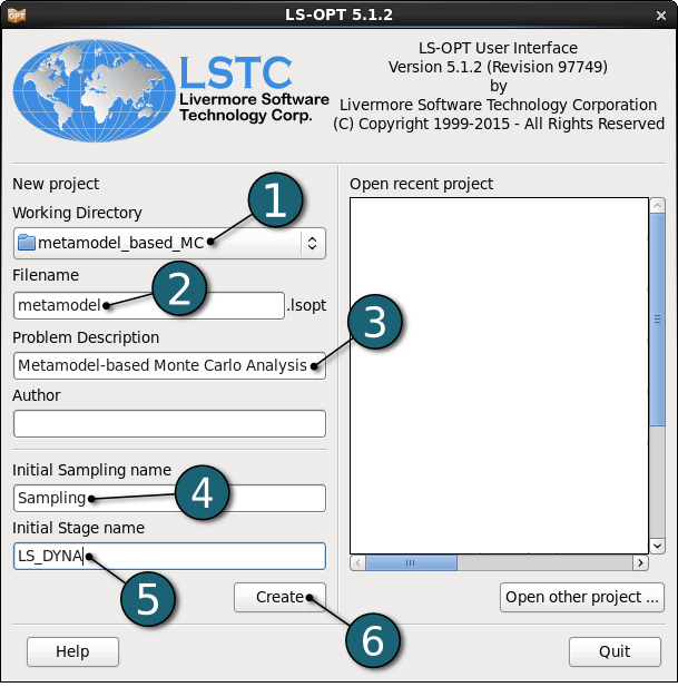
1. Select the Working Directory of the LS-OPT project.
2. Select a suitable name for the file under Filename (e.g. metamodel). The extension .lsopt is appended by LS-OPT.
3. Description of the main task can e.g. be a suitable name for Problem Description ( in this case, Metamodel-based Monte Carlo Analysis, optional).
4. Choose a suitable name under the Initial Sampling name (e.g. Sampling).
5. Choose a suitable name under the Initial Stage name (e.g. LS_DYNA).
6. Click on the Create button to initiate the formation of the input file.

• The main GUI window of LS-OPT opens.

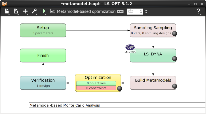
Home Screen Process Flowchart

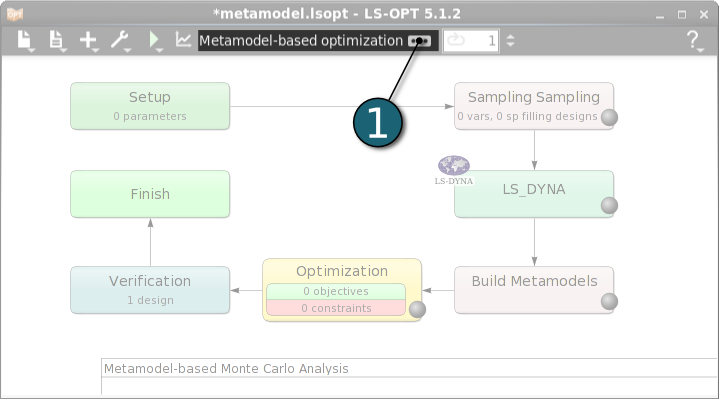
1. Click on the Show task settings icon to select the optimization task and strategy.

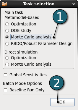
The Task Selection window shall then open.

Define the Main Task

1. Select Monte Carlo analysis as Metamodel-based method.
2. Click on the OK button to proceed.

• After defining the main optimization task the Home Screen Process Flowchart takes its shape accordingly.

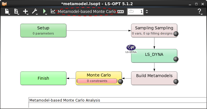
Home Screen Process Flowchart

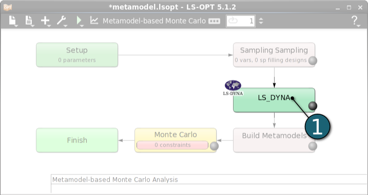
1. Double click on the LS_DYNA box to define the solver stage in the simulation process.

The Stage dialog window shall open.

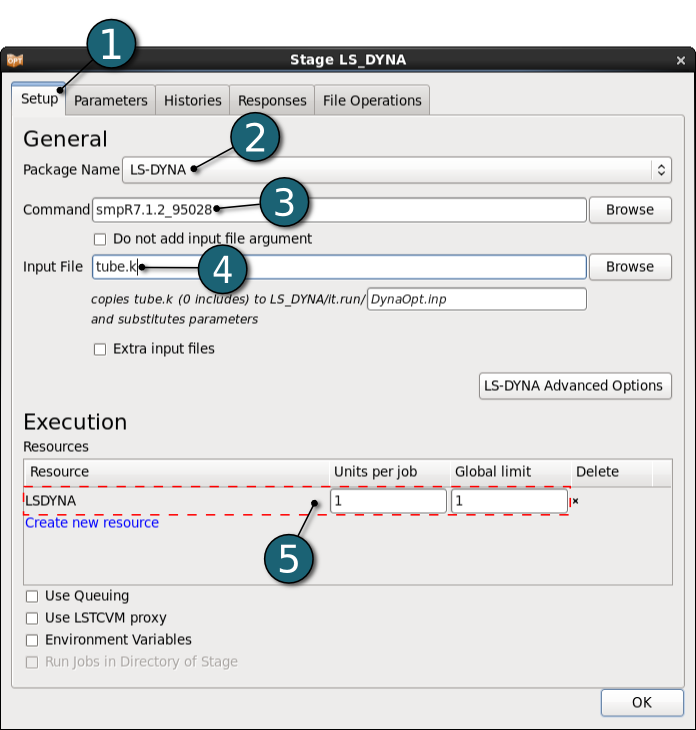
Define Stage Setup

1. Select the Setup tab.
2. Select the solver Package Name as LS-DYNA.
3. For Command enter smpR7.1.2_95028 (or the respective command available on your system). On Windows, the command has to be specified using the absolute path. 
4. For Input File browse the LS-DYNA keyword file tube.k. Parameters are defined in this file by using  LS-DYNA keyword format *PARAMETER.
5. For efficient usage of the computing power from the machine, choice on handling number of concurrent jobs can be made suitable in this section. For more details see FAQ resources.

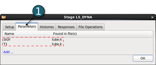
Design Parameters

1. The parameters defined in the selected Input File can be seen in the adjoining tab Parameters.

Define Histories

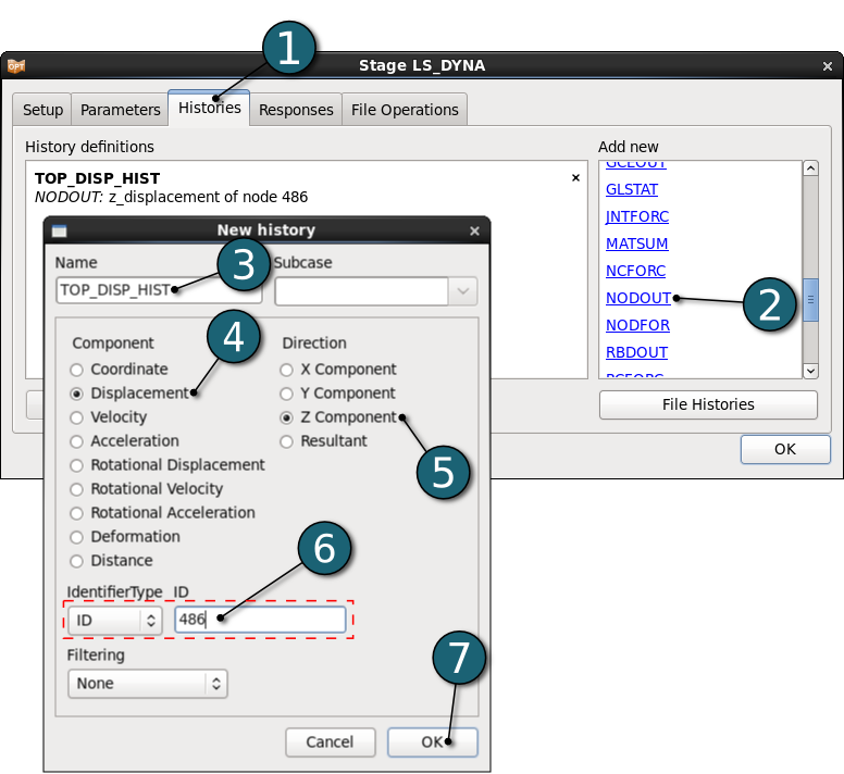
1. Select Histories tab.
2. Select NODOUT as a type of history under the standard LS-DYNA binary database list.
3. Enter TOP_DISP_HIST as the Name of history.
4. Select Displacement as a Component.
5. Select Z Component as a Direction.
6. Select node ID as a Identifier Type and enter 486 as node ID.
7. Click on the OK button to end the history definition.

Define Responses

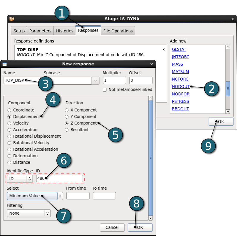
1. Select the Responses tab.
2. Select NODOUT as a type of history under the standard LS-DYNA binary database list.
3. Enter TOP_DISP  as the Name of the response.
4. Select Displacement as a Component.
5. Select Z Component as a Direction.
6. Select node ID as a Identifier Type and enter 486 as node ID.
7. Select the Minimum Value of the displacement of this node in selected z-direction.
8. Click on the OK button to end the response definition.
9. Click on the OK button to proceed.

Home Screen Process Flowchart

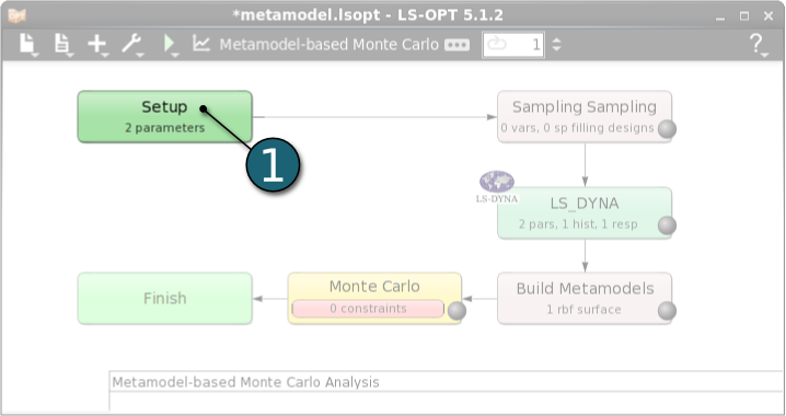
1. Double click on the Setup box for the conversion of parameters to design variables of different types.

The Problem global setup dialog shall open.

Define Parameters

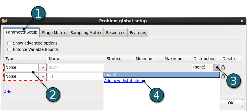
1. Select Parameter Setup tab.
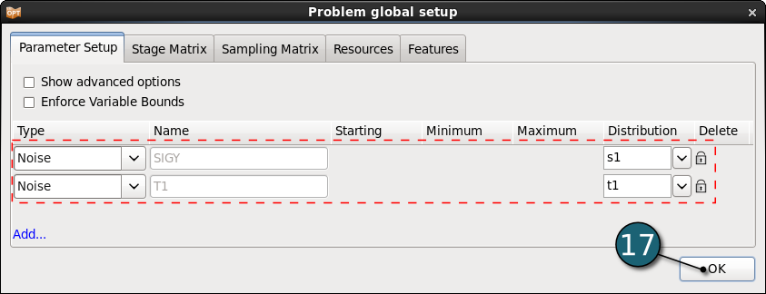
2. Select the Type for both probabilistic design variables as Noise.
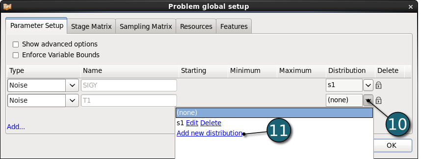
3. Open the Distribution settings dialog to define the distribution of variable SIGY.
4. Click on Add new distribution.
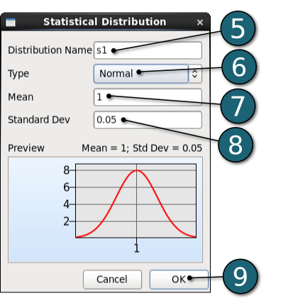
5. Enter s1 as the Distribution Name.
6. Select the distribution Type as Normal.
7. Enter 1 for Mean value.
8. Enter 0.05 for Standard Deviation.
9. Click on the OK button to end the distribution definition for variable SIGY.

10. Open the Distribution settings dialog to define the distribution of variable T1.
11. Click on Add new distribution.
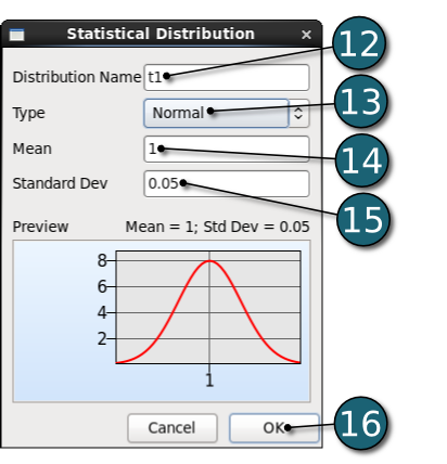
12. Enter t1 as the Distribution Name.
13. Select the distribution Type as Normal.
14. Enter 1 for Mean value.
15. Enter 0.05 for Standard Deviation.
16. Click on the OK button to end the distribution definition for variable T1.
17. Click on the OK button to proceed.

Home Screen Process Flowchart

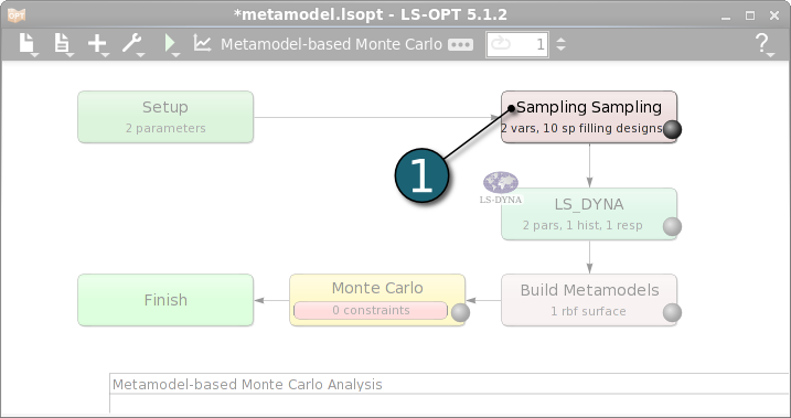
1. Double click on the Sampling box in order to define sampling settings.

A Sampling dialog shall open.

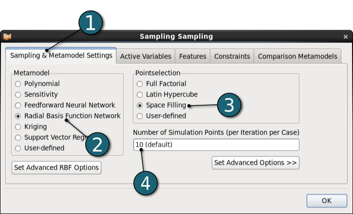
Define Metamodel Settings

1. Select Metamodel Settings tab.
2. Select Radial Basis Function Network as Metamodel type. All statistics will be evaluated on the metamodel, hence we need a good global metamodel.
3. Select Space Filling as Pointselection method.
4. Enter 10 as default for the Number of Simulation Points.
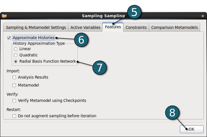
5. Select Features tab.
6. Enable Approximate Histories.
7. Select the History Approximation Type as Radial Basis Function Network.
8. Click on the OK button to proceed.

Home Screen Process Flowchart

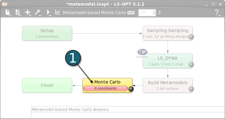
1. Double click on the Monte Carlo box.

The Optimization dialog shall open.

 A Monte Carlo Analysis does not use objective functions, since no optimization is performed, but constraints.

Define Constraints

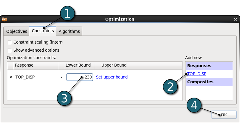
1. Select Constraints tab.
2. Select the response TOP_DISP to be constrained.
3. Set the Lower Bound for this response to -230.
4. Click on the OK button to proceed.

Home Screen Process Flowchart

Run LS-OPT

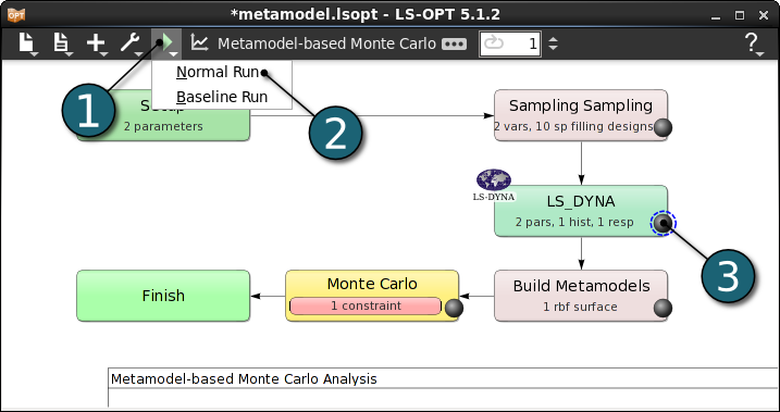
1. Click on the Run button on the Control Bar.
2. Click on the Normal Run.
3. For every stage the user has the option to observe the progress of the program execution by selecting the LED at the corner  on the Stage box. It is possible to observe the Progress and View Log for more information about the execution process.

• Surface
• Accuracy
• Statistical Tools
• Stochastic Contribution
• Histories
• DynaStats

Home Screen Process Flowchart

1. Click on the Open the viewer icon in the contral bar on the Home Screen Process Flowchart window.

A New Plot window shall open.

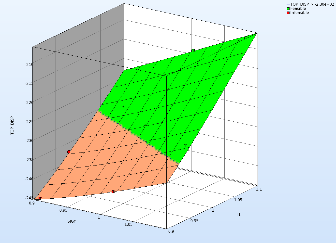
2. Choose Surface under Metamodel.

Surface Plot Settings

1. Select the Setup tab.
2. Select the variables SIGY, T1 and the response TOP_DISP for the x, y and z axis of the plot, respectively.
3. Display the Constraints on the plot.
4. Select the Points tab.
5. Select Current Iteration to display.
6. Display the Feasible and Infeasible points.

 

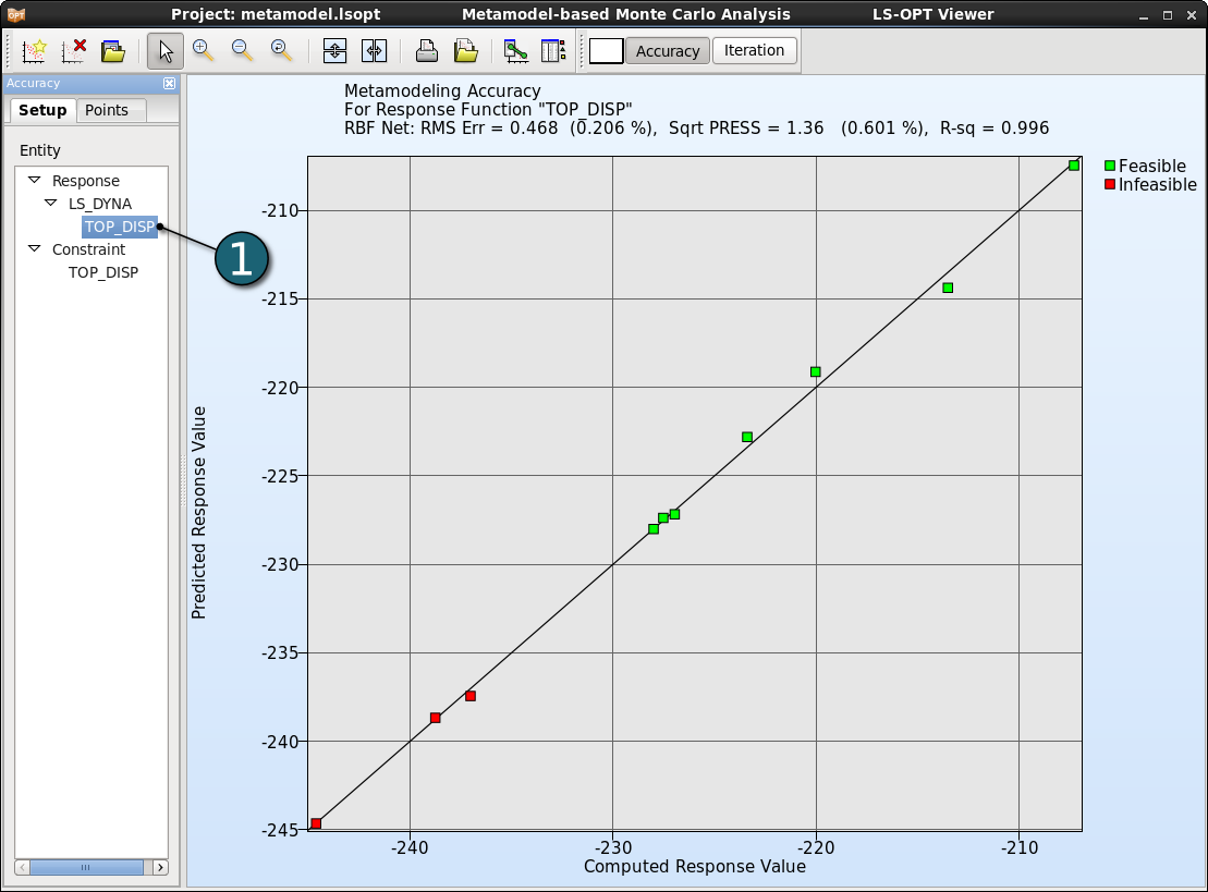
The accuracy of the metamodel fit for the selected response or composite is illustrated in a Predicted vs. Computed plot.

 

New Plot - Accuracy

 

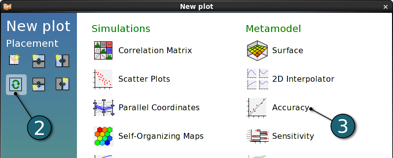
1. Click on the New Plot icon in the menu bar - (or click on the Open the viewer icon on the Home Screen Process Flowchart).

 

A New Plot window shall open.

2. Select Replace current plot icon.
3. Select Accuracy under Metamodel.

Accuracy Plot Settings

1. Select the Response TOP_DISP to displays the accuracy of the metamodel for this response in the Setup tab.

New Plot - Statisctical Tools

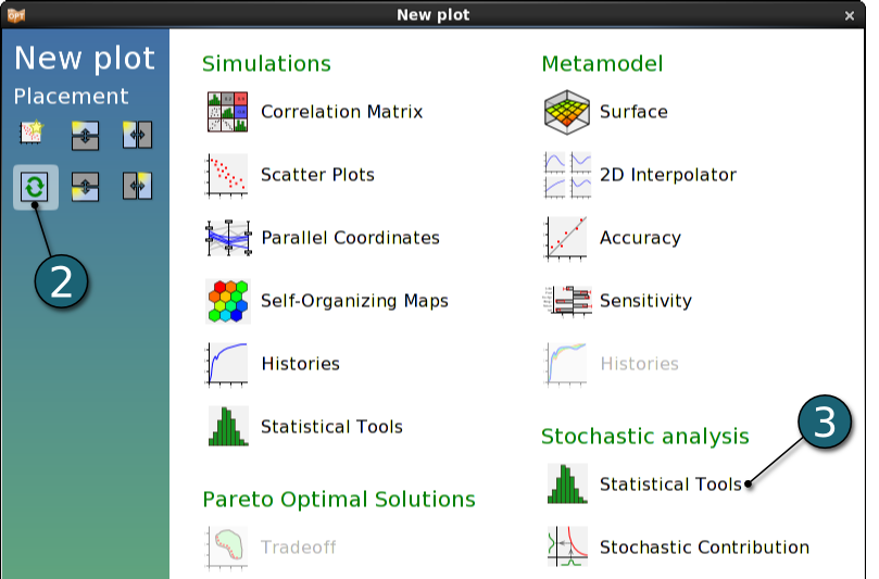
1. Click on the New Plot icon in the menu bar - (or click on the Open the viewer icon on the Home Screen Process Flowchart).

A New Plot window shall open.

2. Select Replace current plot icon.
3. Select Statistical Tools under Stochastic analysis.

Histogram

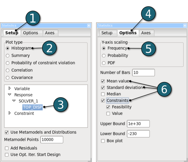
1. Select Setup tab in the new opened Statictical Tools plot window.
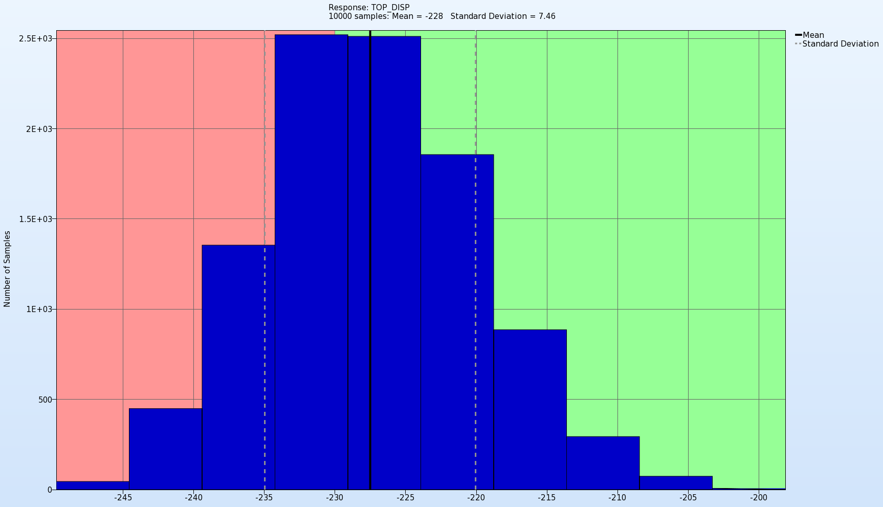
2. Select the Plot type as Histogram.
3. Select the response TOP_DISP to plot its histogram.
4. Select Options tab.
5. Select Frequency as Y-axis scaling.
6. Display Mean Value, Standard deviation and Contraints with Feasibility on the histogram.

 Summary

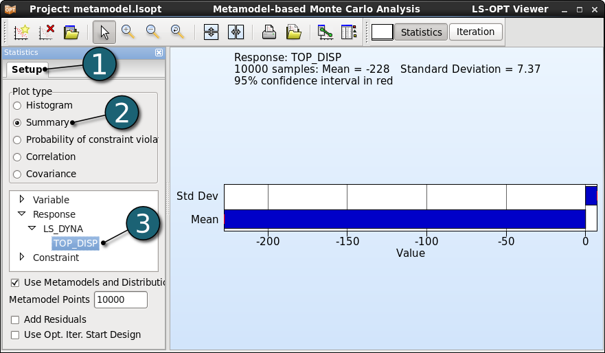
Here, we display the standard deviation and the mean value for the response TOP_DISP with the 95% confidence interval which is shown in red.

1. Select Setup tab.
2. Select the Plot type as Summary.
3. Select the response TOP_DISP whose standard deviation and mean value are shown.

• In this case the confidence intervals are very small, which means the results are very certain.

 Probability of constraint violation

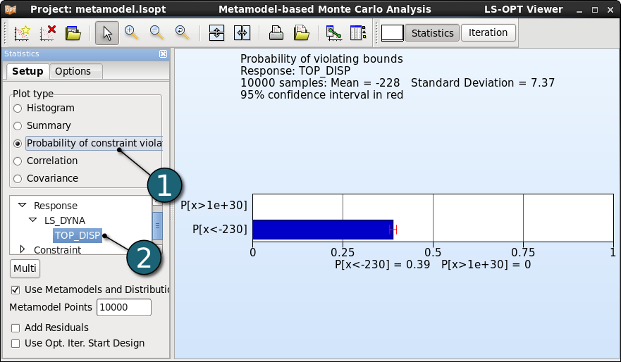
1. Select Probability of constraint violation as a Plot type.
2. Select the response TOP_DIPS.
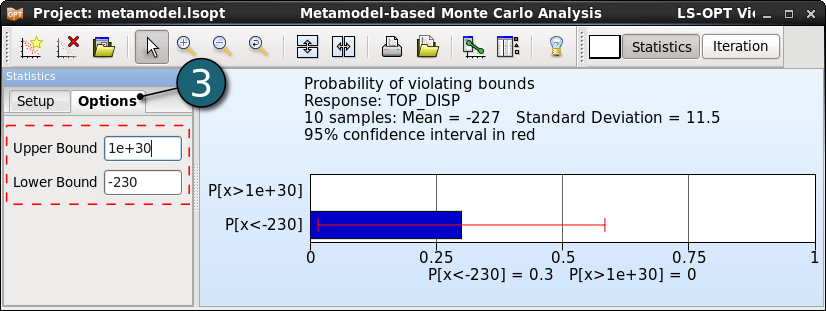
3. We can adjust the upper and lower bounds of the constraint by selecting the Options tab.

•  The 95% confidence interval is shown in red.

Correlation

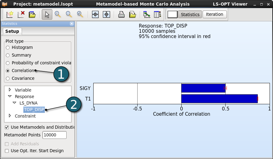
1. Select the Plot type as Correlation.
2. Select the response TOP_DIPS.

 

• The 95% confidence interval is shown in red.

New Plot - Stochastic Contribution

1. Click on the New Plot icon in the menu bar - (or click on the Open the viewer icon on the Home Screen Process Flowchart).

A New Plot window shall open.

2. Select Replace current plot icon.
3. Select Stochastic Contribution under Stochastic analysis.

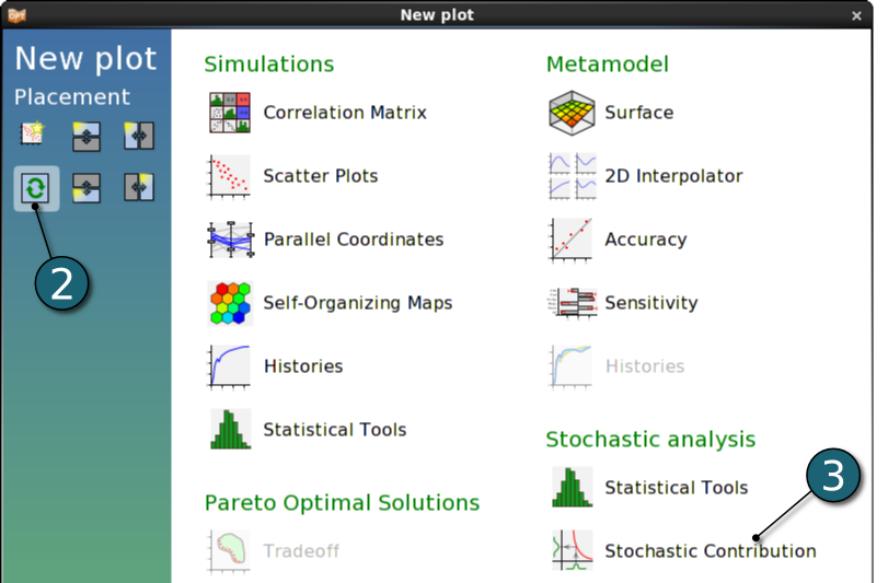
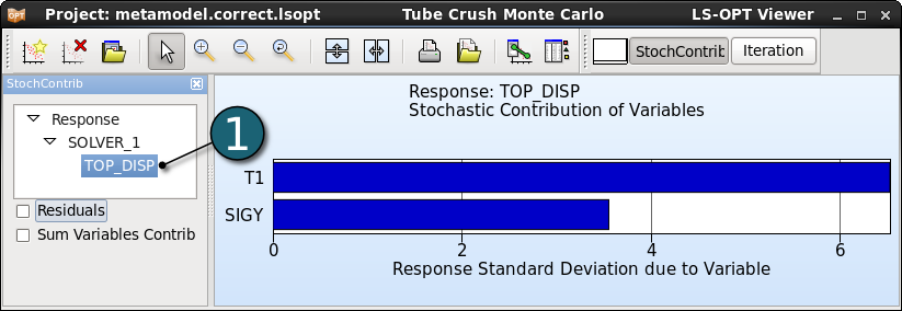
Stochastic Contribution Settings

1. Select the Response TOP_DISP to display the stochastic contribution in the Setup tab.

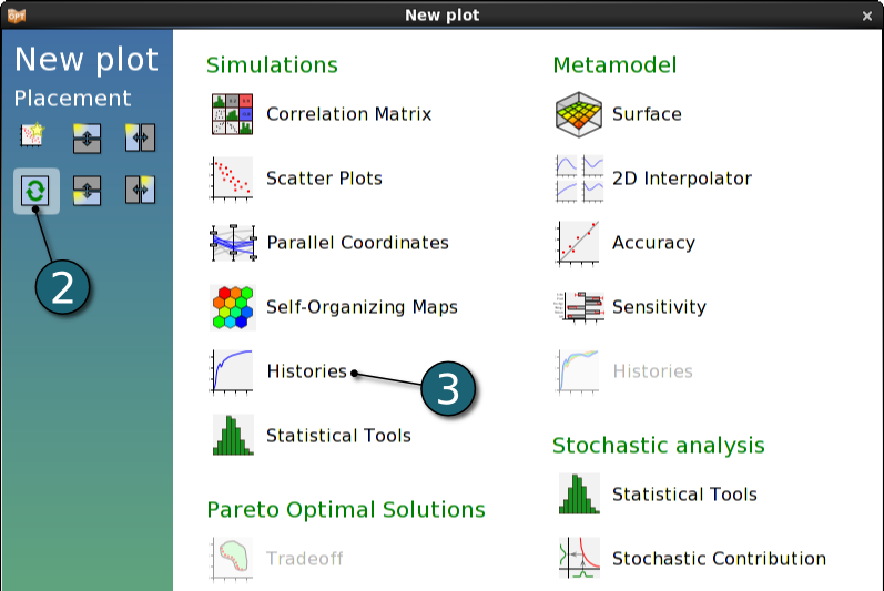
New Plot - Histories

1. Click on the New Plot icon in the menu bar - (or click on the Open the viewer icon on the Home Screen Process Flowchart).

A New Plot window shall open.

2. Select Replace current plot icon.
3. Select Histories under Simulations.

 

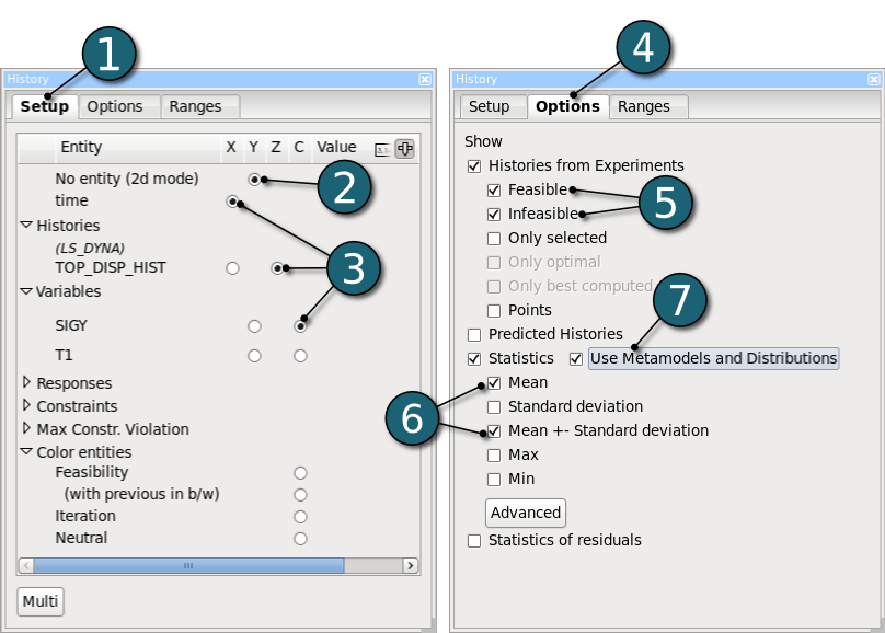
Plot History - Settings

1. Select Setup tab.
2. Select No entity (2d mode) to display history in 2D.
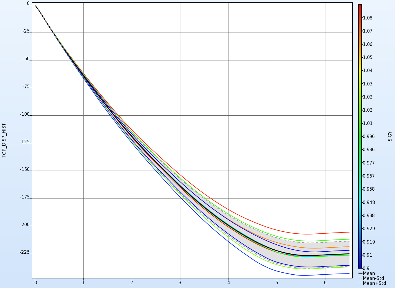
3. Select time, the history TOP_DISP_HIST and the variable SIGY for x-, y- and c- axis, respectively.
4. Select Options tab.
5. Show the Feabisle and Infeasible Histories from the experiments.
6. Show the Mean and Mean+-Standard deviation from Statictics which will be schown in black line and grey dashed line, respectively.
7. Enable Use Metamodels and Distributions.

The statistics of the LS-DYNA results can be displayed on the FE model using DynaStats. The statistics of the LS-DYNA d3plot results and LS-OPT history data are computed by LS-OPT for viewing in LS-PREPOST.
 

Open DynaStats

Home Screen Process Flowchart

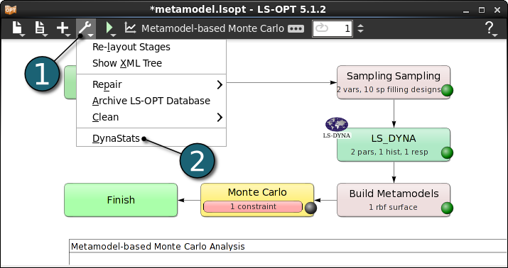
1. Click on the Tools menu of the control bar.
2. Click on the DynaStats.

 

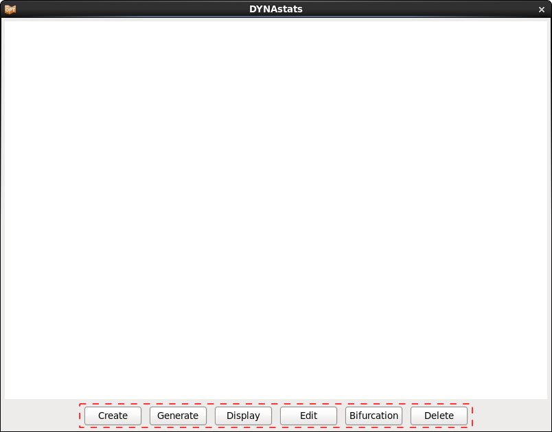
A new DynaStats dialog shall open.Utilize the following actions:

• Create
• Generate
• Display
• Edit
• Bifurcation
• Delete

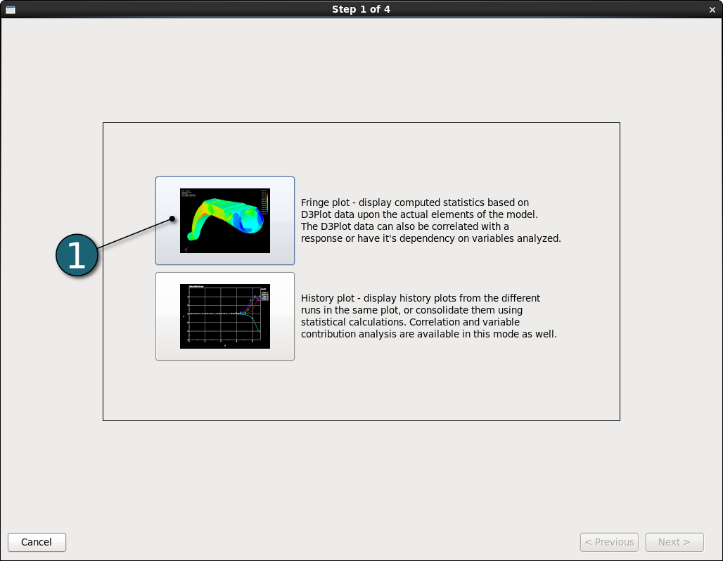
Create Fringe Plot

1. Select Fringe plot option after clicking on the Create button in the main DynaStats dialog.

Display the Statistics in LS-PrePost (D3Plot) - Mean

1. Select z_displacement from the list Ndv (Nodal displacement velocity).
2. Go to the Next panel.

 

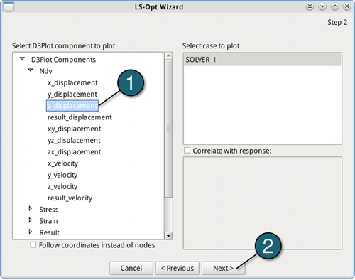
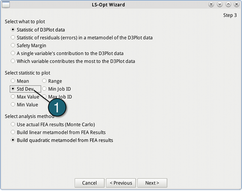
3. For what to plot select Statistic of D3Plot data.
4. Choose Mean as statistic to plot.
5. Build Quadratic Metamodel instead of using actual FEA results.
6. Go to the Next panel.

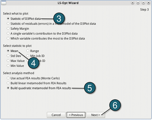
7. Give a name to this plot, e.g. z_disp-mean-quad.
8. Click on the Finish button.

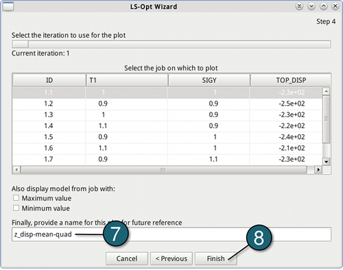
• Select the new created plot z_disp-mean in the DynaStats dialog and then click on the Generate option to generate the data for the plot.
• Display the previously generated plot.
• Metamodels can be used to predict the statistics of the responses. These metamodels (approximations) are computed for all the results for all nodes for all time steps.

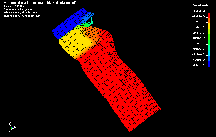
The figure shows the mean of the z-displacement at time 0.99963s.

→ The minimum occurs at node 259 (min=-64.1072) and the maximum at node 429 (max=0.0169754).

Display the Statistics in LS-PrePost (D3Plot) - Standard deviation

• It follows the way explained above, except:

1. By the second step, choose Std Dev (Standard deviation) as statistic to plot.

• Name the plot z_disp-std_dev-quad in the next panel.

 

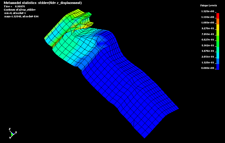
The figure shows the standard deviation of the z-displacement at time 0.99978s.

→ The maximum occurs at node 694 (max = 1.32686) where the deformation is large.

Single variable Mode (Contribution Analysis)

• It follows the way of drawing a fringle plot, but:

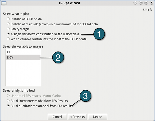
1. By the second step, select A single variable's contribution to the D3Plot data instead of Statistic of D3plot data.
2. Select the variable SIGY.
3. Select quadratic metamodel from FEA result as analysis method.

 

4. In the last step, give a name to this plot, e.g. single_variable.

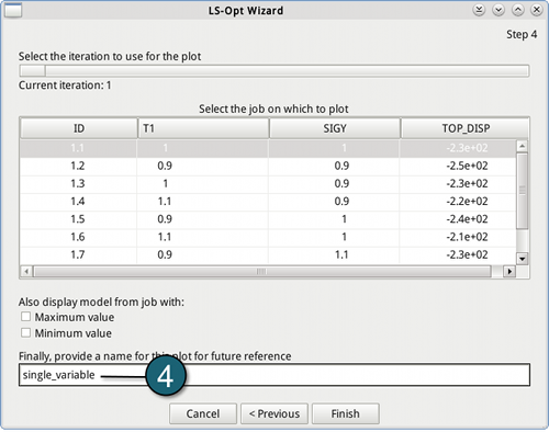
Metamodels can be used to predict the statistics of the responses. In this case the statistics are computed due to one variable (SIGY).

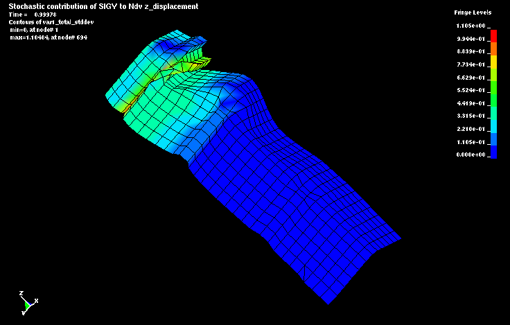
→ The minimum occurs at node 1 (min=0) and the maximum at node 694 (max=1.10725).