Solution with LS-OPT
- Start-up
- Task
- Stage
- Setup
- Sampling
- Composites
- Optimization
- Termination
- Verification
- Run
- Results
- Downloads
Working Directory and Extraction of necessary files
- Create a working directory in the desired location to keep the LS-OPT project file and input files, as well as the LS-OPT program output, e.g. full_vehicle_model.
- Extract all the files required for this example from download section into the working directory.
Project Details
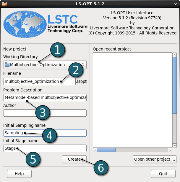
- Select the Working Directory of the LS-OPT project.
- Select a suitable name for the file under Filename (e.g. multiobjective_optimization). The extension .lsopt is appended by LS-OPT.
- Description of the main task can e.g. be a suitable name for Problem Description ( in this case, Metamodel-based multiobjective optimization, optional) .
- Choose a suitable name under the Initial Sampling name (e.g. Sampling).
- Choose a suitable name under the Initial Stage name (e.g. Stage).
- Click on the Create button to initiate the formation of the input file.
- The main GUI window of LS-OPT opens.
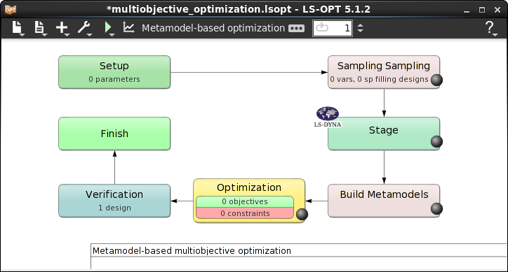
Home Screen Process Flowchart
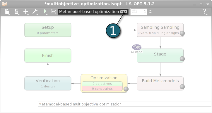
- Click on the Show task settings icon to select the optimization task and strategy.
The Task Selection window shall open.
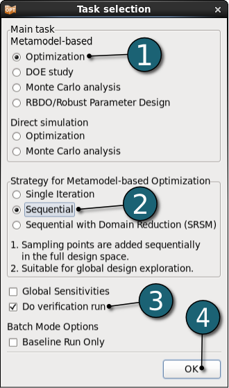
Define the Main Task
- Since a direct optimization requires too many simulations, select the Main task as Metamodel-based Optimization.
- Since the Pareto optimal front requires a global metamodel, select the Sequential optimization strategy.
- Do verification run to execute the predicted optimum design.
- Click on the OK button to proceed.
Home Screen Process Flowchart
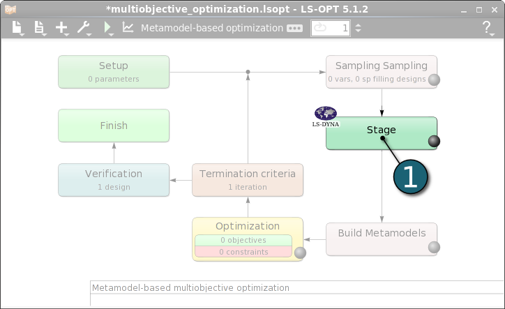
- Double click on the Stage box to define the solver step in the simulation process.
The Stage dialog window shall open.
Define Stage Setup
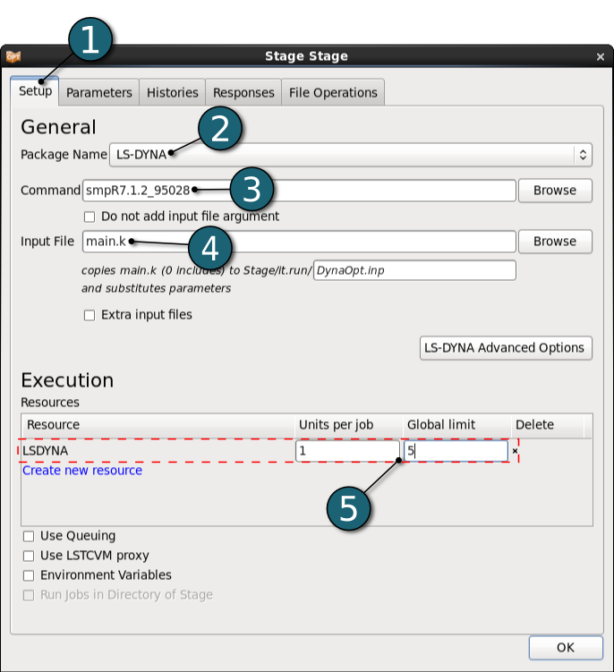
- Select the Setup tab.
- Select the Package Name LS-DYNA.
- For Command enter smpR7.1.2_95028 (This command name can be different on your computer). On Windows, the command has to be specified using the absolute path.
- For Input File browse the LS-DYNA keyword file main.k. Parameters are defined in this file using *PARAMETER keyword. LS-OPT parses this LS-DYNA keyword file automatically for parameters and include files.
- For efficient usage of the computing power from the machine, choice on handling number of concurrent jobs can be made suitable in this section. For more details see FAQ resources.
- The design parameters defined in the input file can be displayed by selecting the Parameters tab in the Stage dialog.
Define Responses
Here we define the system responses some of which are the criteria of interest which are mentioned in the Problem Description.
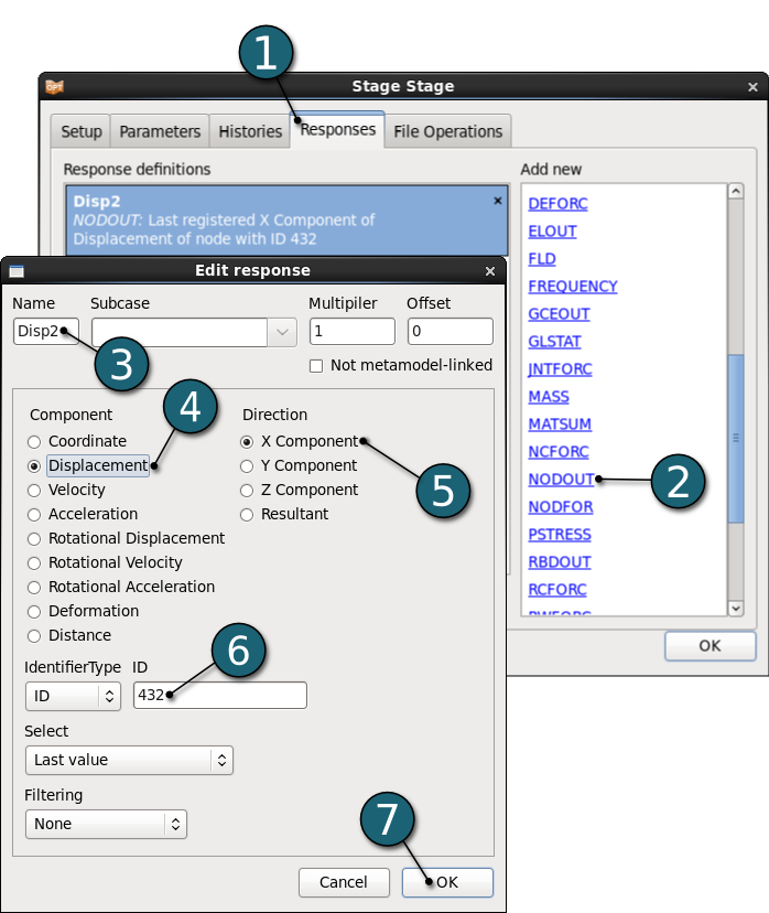
Define the displacement of the node 432
- Select the Responses tab in the stage dialog.
- Select the type of the response as the LS-DYNA binout interface NODOUT from the Add new list on the right side. Edit response dialog will open.
- Enter the Name of the response as Disp2.
- For the Component select Displacement from the list.
- For the Direction select X Component from the list.
- For the node ID enter 432.
- Click on the OK button to end the definition of the response Disp2.
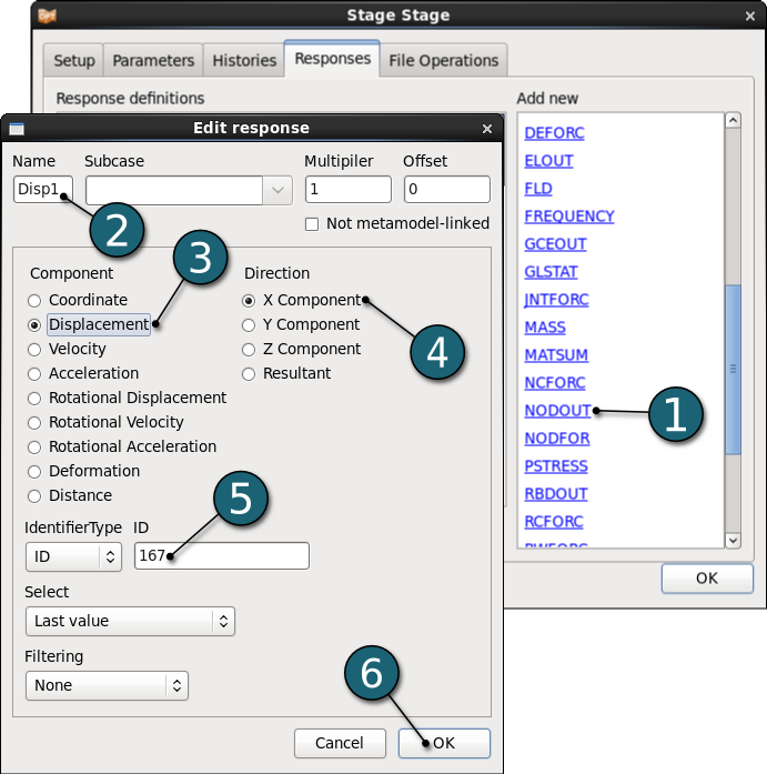
Define the displacement of the node 167
- Select the type of the response as the LS-DYNA binout interface NODOUT from the Add new list. Edit response dialog will open.
- Enter the Name of the response as Disp1.
- For the Component select Displacement from the list.
- For the Direction select X Component from the list.
- For the node ID enter 167.
- Click on the OK button to end the definition of the response Disp1.
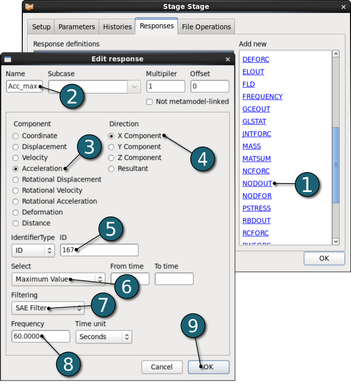
Define the maximum acceleration of node 167
- Select the type of the response as the LS-DYNA binout interface NODOUT from the Add new list. Edit response dialog will open.
- Enter the Name of the response as Acc_max.
- For the Component select the Accelaration.
- For the Direction select X Component.
- For the node ID enter 167.
- Select the Maximum Value of the acceleration of this node.
- Set the Filtering as SAE Filter.
- Enter the Frequency as 60.0000 Seconds.
- Click on the OK button to end the definition of the response Acc_Max.
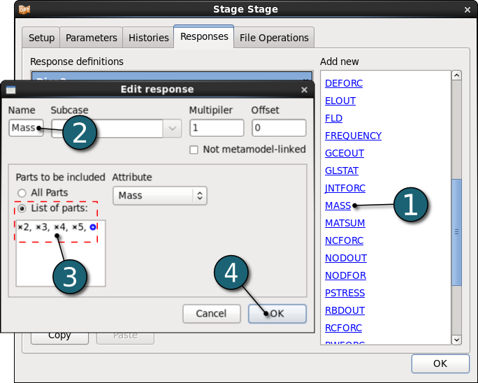
Define Mass
- Select the type of the response as the LS-DYNA d3hsp interface MASS from the Add new list. Edit response dialog will open.
- Enter the Name as Mass.
- Enter the the List of Parts as 2, 3, 4 and 5.
- Click on the OK button to end the definition of the response Mass.
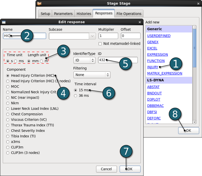
Define HIC
- Select the type of the response as INJURY from the Add new list. Edit response dialog will open.
- Enter the Name as HIC.
- Set the Time unit to s and Legth unit to mm.
- For the Component select the Head Injury Criterion (HIC).
- For the node ID enter 432.
- Select the Time interval as 15 ms.
- Click on the OK button to end the definition of the response HIC.
- Click on the OK button to proceed.
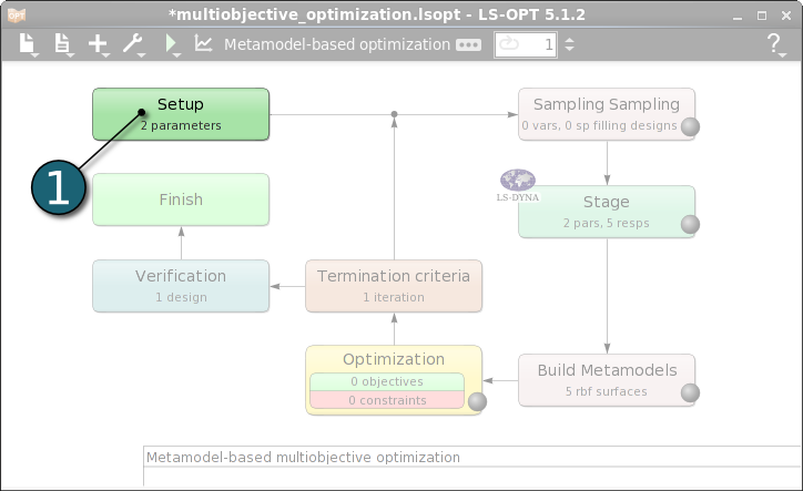
Home Screen Process Flowchart
- Double click on the Setup box for the conversion of parameters in input files to design variables of different types.
The Problem global setup dialog shall open.
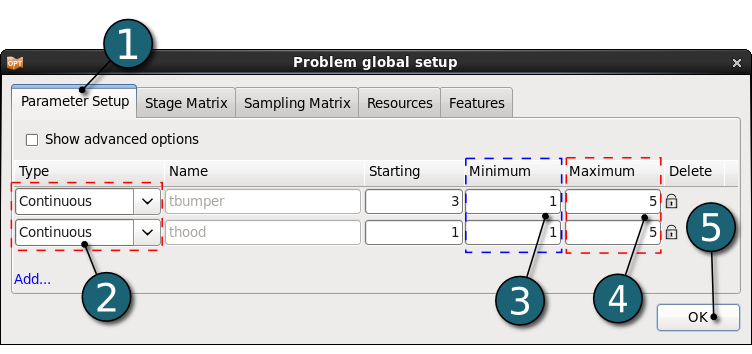
Define Parameters
- Select the Parameter Setup tab.
- Select the variable Type of both parameters tbumper and thood as Continuous.
- Set the Minimum values of both parameters to 1.
- Set the Maximum values of both parameters to 5.
- Click on the OK button to proceed.
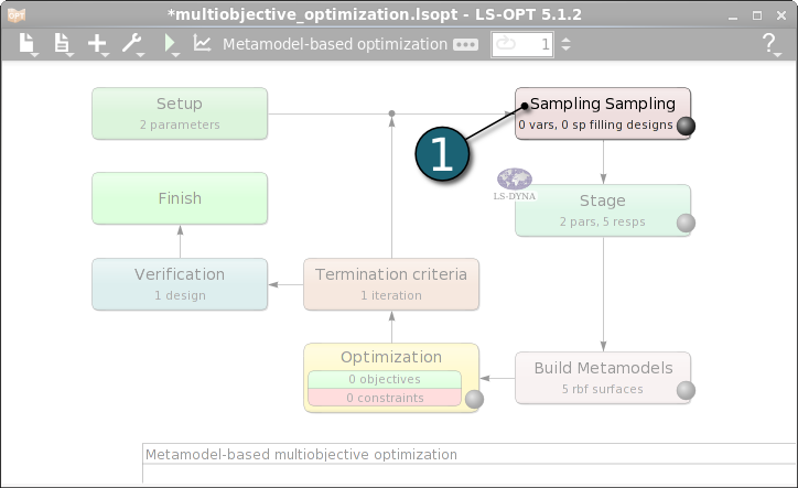
Home Screen Process Flowchart
- Double click on the Sampling Direct box in order to define sampling settings.
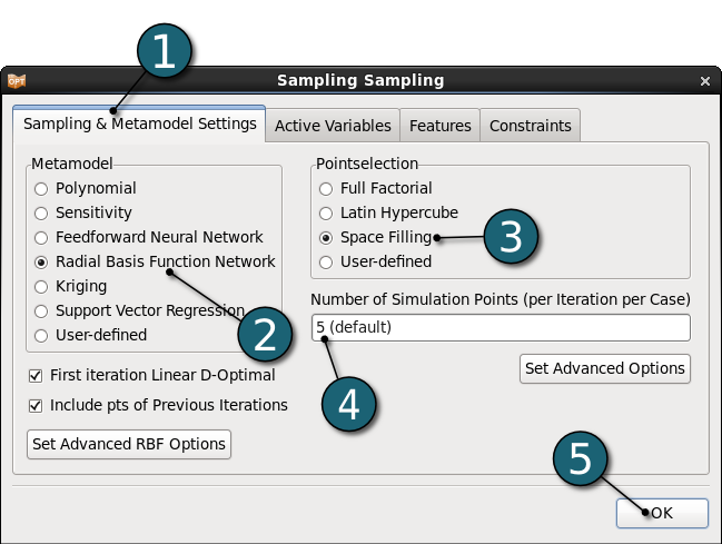
A Sampling dialog shall open.
Define Sampling Settings
- Select Sampling & Metamodel Settings tab.
- Select the Metamodel type as Radial Basis Function Network.
- Select the Pointselection method as Space FIlling.
- Enter the Number of Simulation Points as default 5.
- Click on the OK button to proceed.
Home Screen Process Flowchart
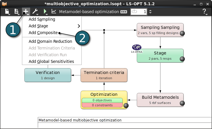
Add Composite
- Click on the Add menu in the control bar.
- Select Add Composite from the Add list.
A Composites dialog shall open.
Define Composites
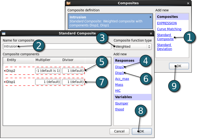
- Select the type of composite as Standard Composite in the Composites list to define Intrusion = Disp1 - Disp2.
- Enter the Name as Intrusion.
- Select Composite function type as Weighted.
- Select the response Disp2.
- Set the Multiplier to -1 and the Divisor as default 1 for Disp2.
- Select the response Disp1.
- Set the Multiplier to -1 and the Divisor as default 1 for Disp1.
- Click on the OK button to end the definition of the composite.
- Click on the OK button to proceed.
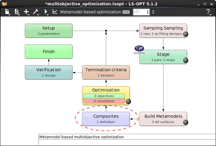
- After defining composite expression the Composite box takes its place in the Home Screen Process Flowchart.
Home Screen Process Flowchart
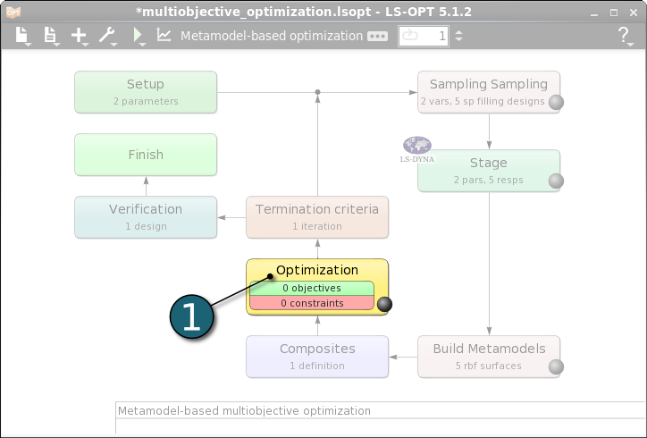
- Double click on the Optimization box to specify objectives and constraints for the design formulation and the optimization algorithm.
The Optimization dialog shall open.
Define Objectives
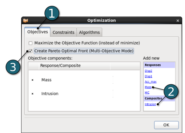
- Select the Objectives tab.
- Select the objectives as the response Mass and the composite Intrusion from Add new list on the right side.
- Activate Create Pareto Optimal Front (Multi-Objective Mode). Pay attention that this option is only available if at leaset two objectives are defined.
Define Constraints
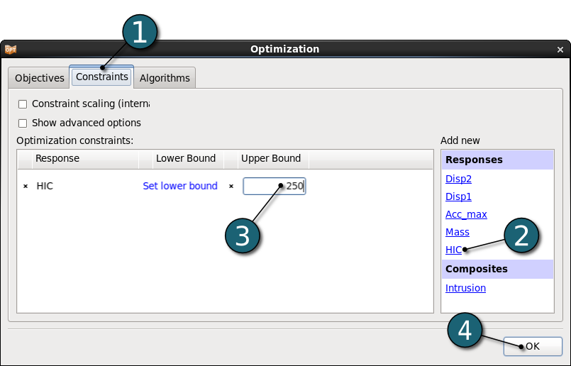
- Select the Constraints tab.
- Select the constraint as the response HIC from Add new list on the right side.
- Set the Upper Bound for HIC to 250.
- Click on the OK button to proceed.
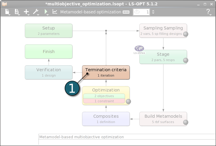
Depending on the optimization task and strategy, the user can specify tolerances on the design change, the objective function change or the accuracy of the metamodel. The user can also specify whether termination is reached if any one, or all of these criteria are met. For the sequential strategy, only the resposne accuracy tolerance is available.
Home Screen Process Flowchart
- Double click on the Termination criteria box.
A Termination Criteria dialog will open.
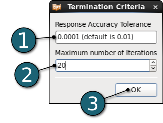
Define Termination Criteria
- Enter 0.0001 for the Response Accuracy Tolerance.
- Enter 20 for the Maximum number of iterations.
- Click on the OK button to proceed.
After the last full iteration verifications run of selected predicted Pareto optimal designs can be executed. Those runs can also be omitted if the user is only interested in the prediction of the Pareto optimal solutions evaluated on the metamodel.
A discrete Space Filling algorithm is used to select Pareto Optimal points which are evenly distributed in the design space.
Home Screen Process Flowchart
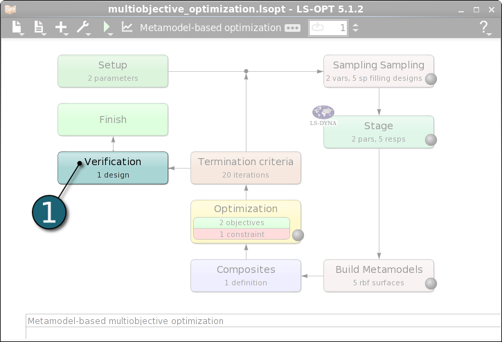
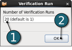
- Double click on the Verification box.
A Verification Run dialog will open.
Define Termination Criteria
- Enter 20 for the Number of Verification Runs.
- Click on the OK button to proceed.
Home Screen Process Flowchart
Run LS-OPT
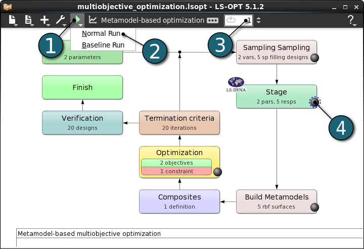
- Click on the Run button on the Control Bar.
- Click on the Normal Run.
- The user can get information on the status of the current iteration during execution.
- For every stage the user has the option to observe the progress of the program execution by selecting the LED at the corner on the Stage box. It is possible to observe the Progress and View Log for more information about the execution process.
Home Screen Process Flowchart
- Click on the Open the viewer icon in the control bar on the Home Screen Process Flowchart.
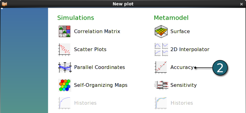
A New Plot window shall open.
- Select Accuracy under the Metamodel.
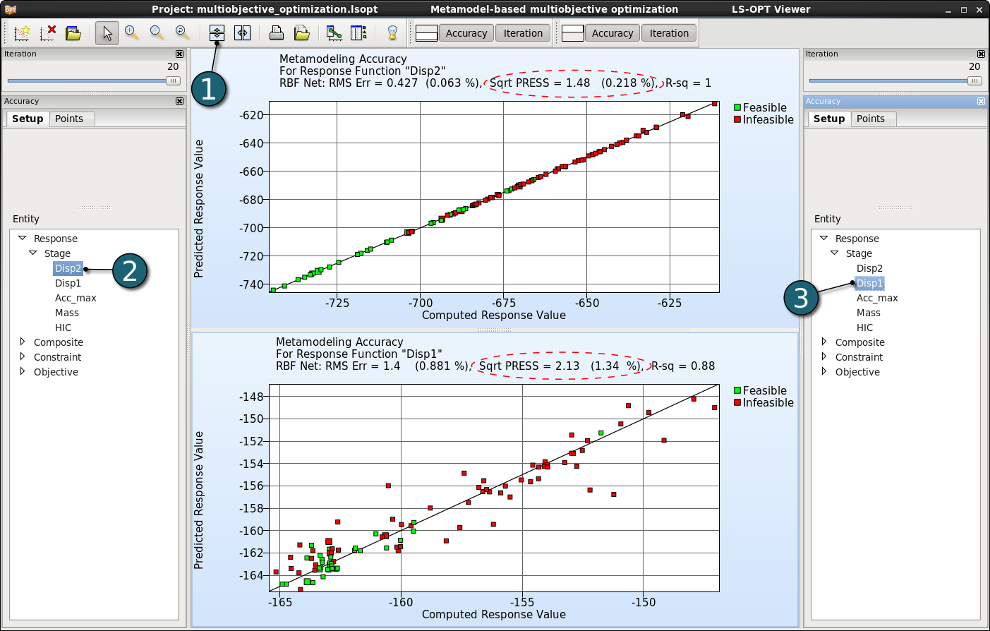
Since the Pareto optimal solutions are evaluated on the global metamodel, the quality of the metamodel is important.

Accuracy Plot Settings
- Click on the Split vertical button to display the accuracies of the metamodel for the responses Disp1 and Disp2.
- Select Disp2 for the first plot.
- Select Disp1 for the second plot.
- The predicted and computed values are very close to each other. The SPRESS errors are also displayed on each accuracy plot. 0.218% and 1.34% errors are pretty much acceptable.
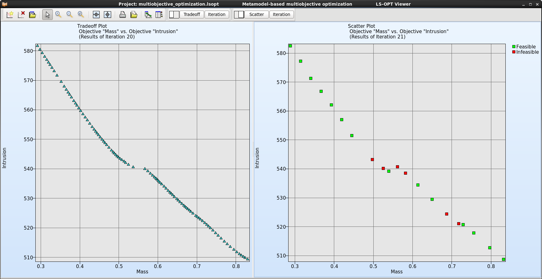
The Tradeoff plot functions similar to the Scatter plot, but the default setting is here to plot Pareto optimal solution data instead of Analysis Result data.
New Plot - Tradeoff- Click on the New Plot icon in the menu bar - (or click on the Open the viewer icon on the Home Screen Process Flowchart).
- Select Replace current plot icon.
- Select Tradeoff under Perato Optimal Solutions.

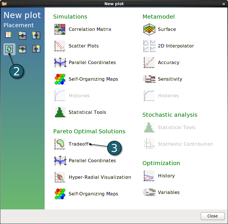
- Tradeoff
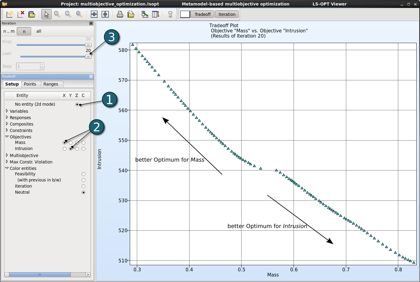
- Display the Pareto front of the optimal solution in 2D.
- As default the objectives Mass and Intrusion are selected for the x and y axes, respectively.
- Display the Pareto optimal solutions for the last iteration 20.
- Each point represents a Pareto optimal solution. As we can see for the best optimum for an objective the other one has the worst optimum. According to the problem we need to choose one of these optimal solutions.
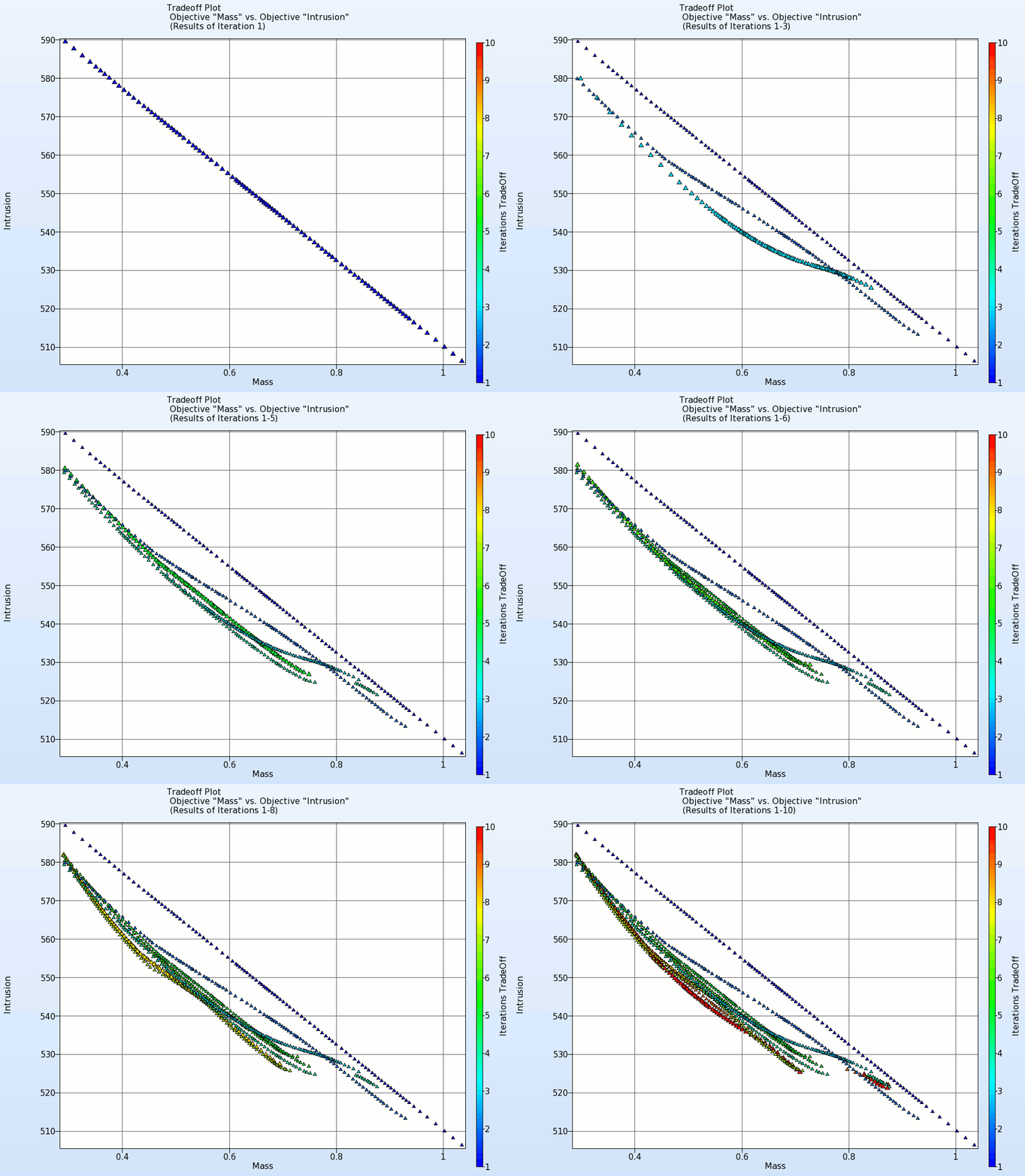
- The animation below shows the development of the Pareto front for the first 10 iterations.
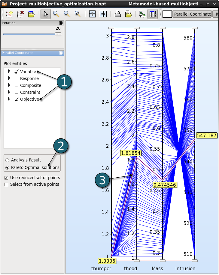
The number of dimensions that can be visualized using the Parallel Coordinate Plot is not restricted. Each dimension is visualized on a vertical axis and each data point is shown as a poly-line connecting the respective values on the vertical axis. Here we use the Parallel Coordinate plot to evaluate the Pareto optimal solutions.
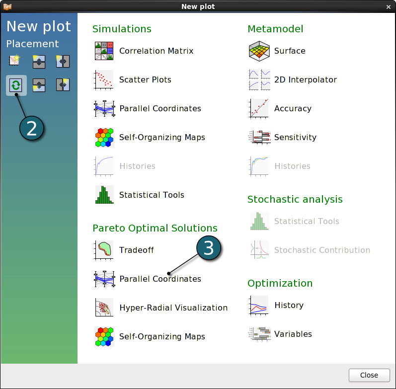
New Plot - Parallel Coordinates
- Click on the New Plot icon in the menu bar - (or click on the Open the viewer icon on the Home Screen Process Flowchart).
A New Plot window shall open.
- Select Replace current plot icon.
- Select Parallel Coordinates under Pareto Optimal Solutions.

Parallel Coordinates Settings
- Select the Plot entities as the both design variables and the both objectives.
- Select Pareto Optimal solutions.
- Selected points are colored in purple. If only a single point is selected, the corresponding value for each entity is displayed in the plot.
Adjusting the Ranges
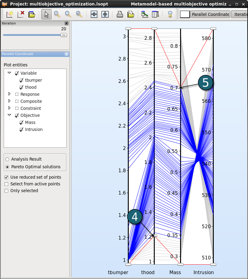
The ranges of the entities may be changed interavtively using the sliders at the ends of each vertical axis rendering the points outside the ranges unselectable. Points within the selected ranges are colored in blue, while the remaining points are colored in grey.
- Changing the lower bound of an entity.
- Changing the upper bound of an entity.
- We may easily reduce the data by adapting the ranges of all entities interactively, what is helpful in decision making.
- But the parallel coordinate plot offers no information on the trends.
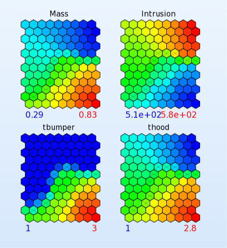
Visualization using Self Organizing Maps is a convenient tool to determine conflicting objectives and discontinuities in the Pareto optimal front.
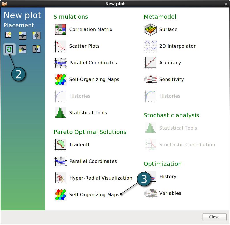
New Plot - Self Organizing Maps
- Click on the New Plot icon in the menu bar - (or click on the Open the viewer icon on the Home Screen Process Flowchart).
A New Plot window shall open.
- Select Replace current plot icon.
- Select Self-Organizing Maps under Pareto Optimal Solutions.

Self-Organizing Maps Settings
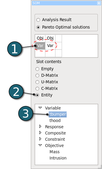
- Select the cell under the first objective. i.e the cell 2x1.
- Select Entity.
- Select the Entity as the variable tbumper.
- Repeat the steps 4-5 for the cell 2x2 and for the variable thood.
- Visualization using Self Organizing Map is a convenient tool to determine conflicting objectives and and objecitves that are in agreemnt, and also the relation between variables and objectives or constraints, respectively.
For Linux : multiobjective_optimization.tar.gz (29.4 kB)
For Windows : multiobjective_optimization.zip (30.3 kB)
