Solution with LS-OPT
Working Directory and Extraction of necessary files
- Create a working directory in the desired location to keep the LS-OPT project file and input files, as well as the LS-OPT program output, e.g. full_vehicle_model.
- Extract all the files required for this example from download section into the working directory.
Project Details
- Select the Working Directory of the LS-OPT project.
- Select a suitable name for the file under Filename (e.g. metal_forming). The extension .lsopt is appended by LS-OPT.
- Description of the main task can e.g. be a suitable name for Problem Description ( in this case, Metal forming optimization, optional) .
- Choose a suitable name under the Initial Sampling name (e.g. Sampling).
- Choose a suitable name under the Initial Stage name (e.g. Forming).
- Click on the Create button to initiate the formation of the input file.
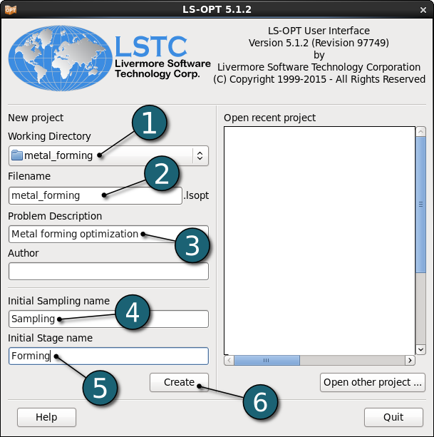
- The main GUI window of LS-OPT opens.
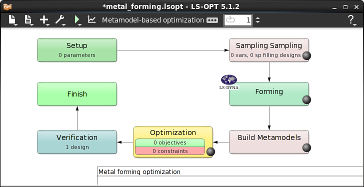
Home Screen Process Flowchart
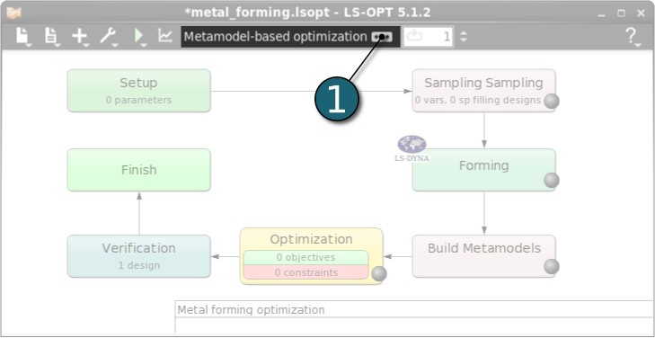
- Click on the Show task settings icon to select the optimization task and strategy.
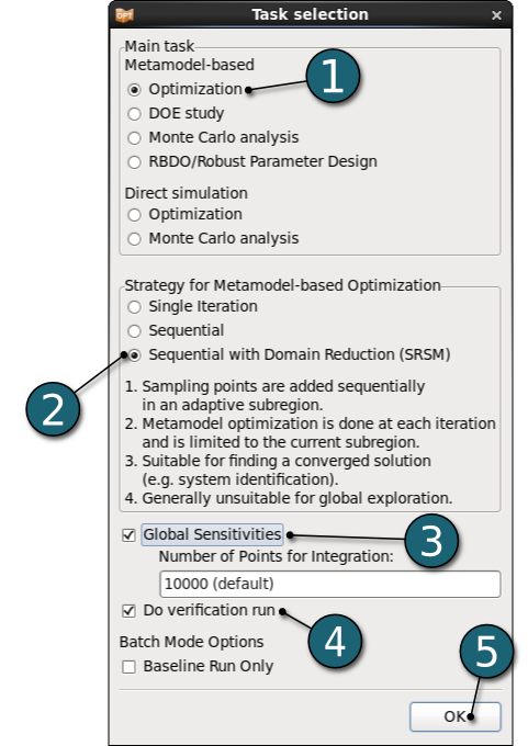
The Task Selection window shall then open.
Define the Main Task
- Select Optimization for the Metamodel-based main task.
- Select Sequential with Domain Reduction (SRSM) as the strategy for the metamodel-based optimization.
- In order to study Global Sensitivities on the metamodel tick the adjacent box. The default number of sampling points for Monte-Carlo integration is 10000. For better accuracy of sensitivity coefficients this number should be increased.
- Activate Do verification run to execute the predicted optimal design after the last full iteration.
- Click on the OK button to proceed.
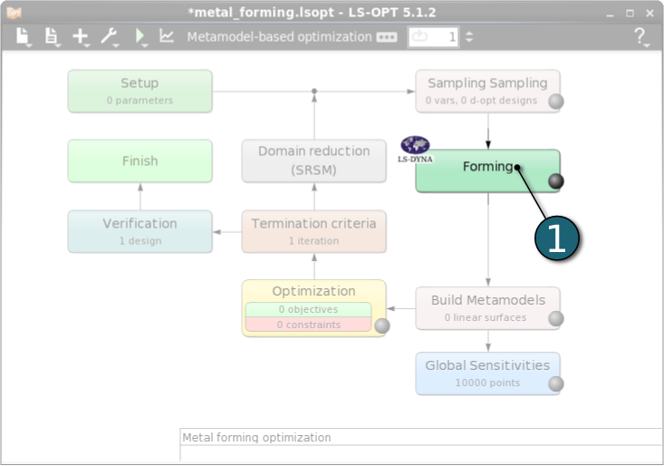
Home Screen Process Flowchart
- Double click on the Forming box to define the solver step in the simulation process.
The Stage dialog window shall open.
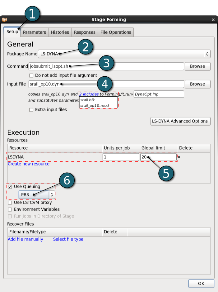
Define Stage Setup for Forming
- Select the Setup tab.
- Select the Package Name LS-DYNA.
- For Command specify jobsubmit_lsopt.sh (This is a script that submits the LS-DYNA jobs to a cluster and needs to be replaced by an appropriate command available on your system).
- For Input File browse the LS-DYNA keyword file srail_op10.dyn. Parameters are defined in this file using *PARAMETER keyword. LS-OPT parses this LS-DYNA keyword automatically for parameters and includes.
- For efficient usage of the computing power from the machine, choice on handling number of concurrent jobs can be made suitable in this section. For more details see FAQ resources.
- In case you run the LS-DYNA jobs on a cluster, activate Use Queuing and select the respective queuing system, e.g. PBS, for interfacing with load sharing facilities to enable running simulation jobs across a network.
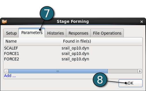
- The parameters defined in the selected Input File can be visualized in the adjoining tab Parameters.
- Since no histories or responses need to be extracted for this stage, click on the OK button to proceed.
Home Screen Process Flowchart
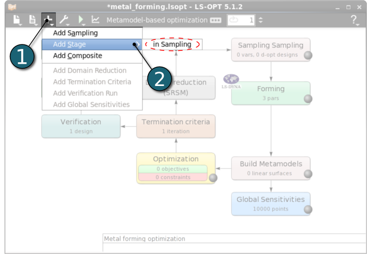
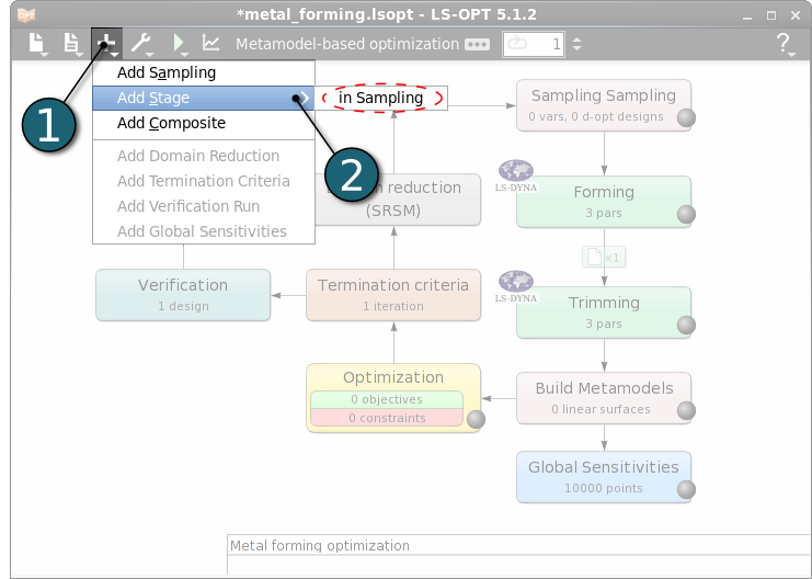
Add Stage
- Click on the Add menu in the control bar.
- Select Add Stage --> in Sampling Sampling for the second step Trimming in the metal forming process.
Enter Trimming as the Name for new stage.
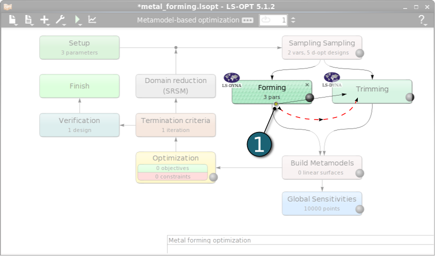
Dependencies of Stages
- The dependency of the stages is set by dragging the arrow head from the stage Forming to the stage Trimming.
- After connecting the two stages to each other we can re-position the stage Trimming for the sake of nice view of flowchart by dragging with simple left-mouse click, or use the Re-layout Stages option from the Tools menu.
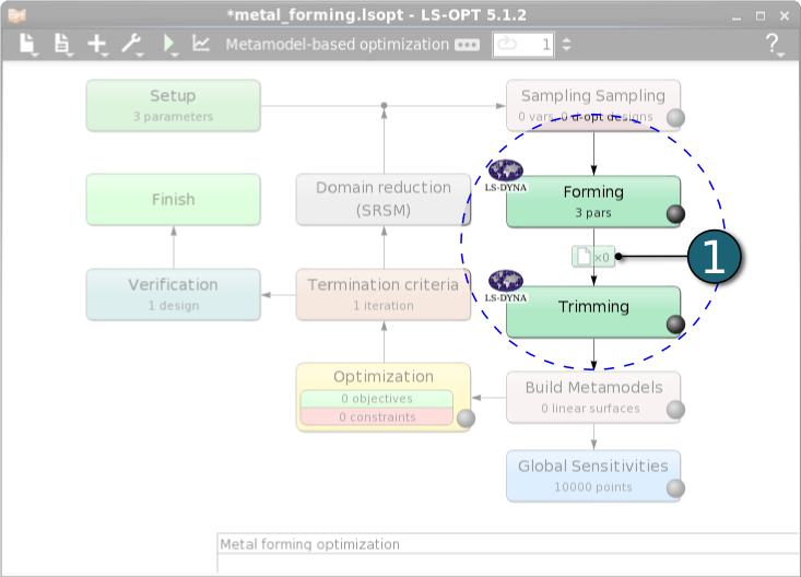
File Transfers
- Since the stage Trimming uses the output file of the stage Forming as an input file, the definition of a file transfer is necessary. Click on the File Transfers icon between the two stages. Another option to make the files available for the Trimming stage is to use the Run in directroy of stage option in the Stage dialog Setup tab.
The File Transfers dialog will open.
- Select the file transfer Operation as Copy.
- Enter the name of the Source File, which is dynain in this case.
- Enter the name of the Destination File, which is dynain in this case, too.
- In the case the operations fails (on Error) select the operation to be applied as fail. The job will return an error termination and LS-OPT won't run the downstream stages for this sampling point.
- Click on the OK button to proceed.

Define Solver Setup for Trimming
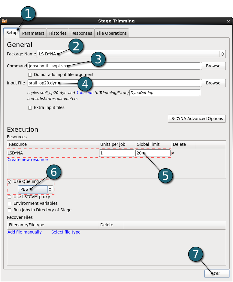
- Open the Trimming - Stage dialog as done for the previous Stage - Forming by double clicking on it. Then select the Setup tab.
- Select the Package Name LS-DYNA.
- For Command specify jobsubmit_lsopt.sh (This is a script that submits the LS-DYNA jobs to a cluster and needs to be replaced by an appropriate command available on your system).
- For Input File browse the LS-DYNA keyword file srail_op20.dyn.
- For efficient usage of the computing power from the machine, choice on handling number of concurrent jobs can be made suitable in this section. For more details see FAQ resources.
- In case you run the LS-DYNA jobs on a cluster, activate Use Queuing and select the respective queuing system, e.g. PBS, for interfacing with load sharing facilities to enable running simulation jobs across a network.
- Click on the OK button to proceed.
Home Screen Process Flowchart
Add Stage
- Click on the Add menu in the control bar.
- Select Add Stage --> in Sampling Sampling for the third step Springback in the metal forming process.
Enter Springback as the Name for new stage.
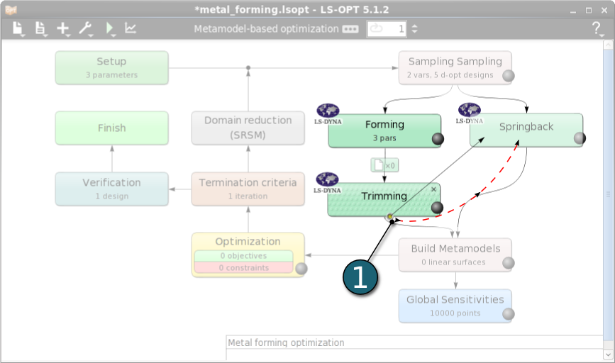
Dependencies of Stages
- The dependency of the stages is set by dragging the arrow head from the stage Trimming to the stage Springback.
- After connecting the two stages to each other we can re-position the stage Springback for the sake of nice view of flowchart by dragging with simple left-mouse click, or use the Re-layout Stages option from the Tools menu..
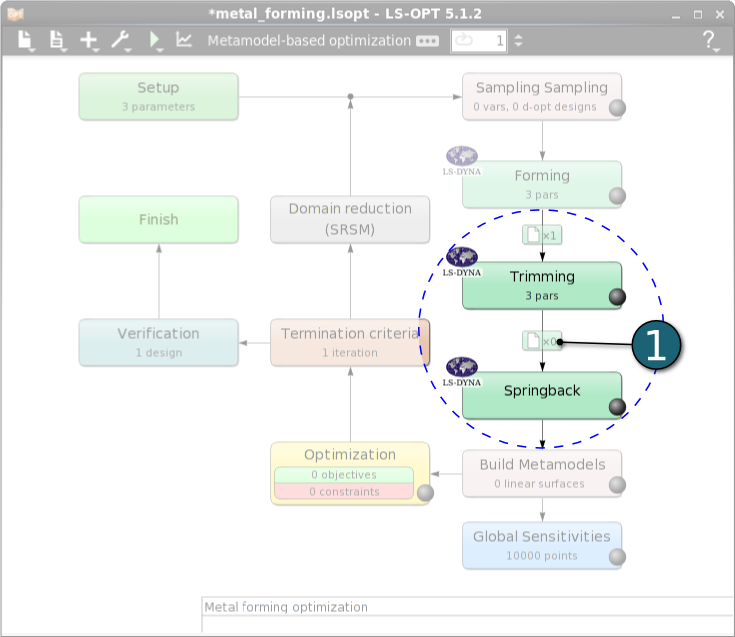
File Transfers
- Since the stage Springback uses the output file of the stage Trimming as an input file, the definition of a file transfer is necessary. Click on the File Transfers icon between the two stages. Another option to make the files available for the Timming stage is to use the Run in directroy of stage option in the Stage dialog Setup tab.
A File Transfers settings dialog will open.
- Select the file transfer Operation as Copy.
- Enter the name of the Source File, which is dynain in this case.
- Enter the name of the Destination File, which is dynain in this case, too.
- In the case the operations fails (on Error) select the operation to be applied as fail. The job will return an error termination and LS-OPT won't run the downstream stages for this sampling point.
- Click on the OK button to proceed.

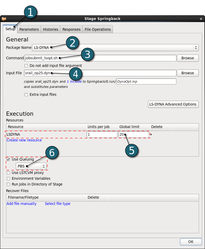
Define Solver Setup for Springback
- Open the Springback - Stage dialog as done for the previous Stage - Forming by double clicking on it. Then select the Setup tab.
- Select the Package Name LS-DYNA.
- For Command specify jobsubmit_lsopt.sh (This is a script that submits the LS-DYNA jobs to a cluster and needs to be replaced by an appropriate command available on your system).
- For Input File browse the LS-DYNA keyword file srail_op25.dyn.
- For efficient usage of the computing power from the machine, choice on handling number of concurrent jobs can be made suitable in this section. For more details see FAQ resources.
- In case you run the LS-DYNA jobs on a cluster, activate Use Queuing and select the respective queuing system, e.g. PBS, for interfacing with load sharing facilities to enable running simulation jobs across a network.
Define Responses
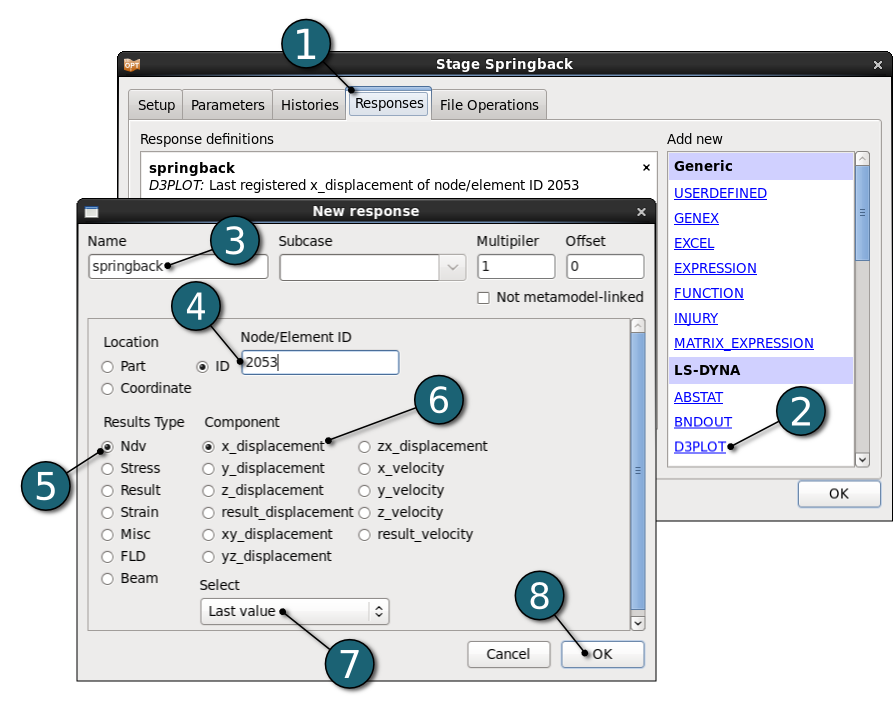
Define springback
- Select the Responses tab.
- Select D3PLOT as the type of response which is produced by LS-DYNA simulation.
- Enter springback as the Name of the response.
- Select ID to specify the Location for the response and enter the Node ID 2053.
- Select the Result Type for this node as Ndv (Nodal Displacement, Velocity etc.).
- Select x_displacement as Component to observe springback in this direction.
- Select Last Value of the nodal displacement in x-direction to find out the resulting springback at the end.
- Click on the OK button to end the response definition.
Define thickness_reduction
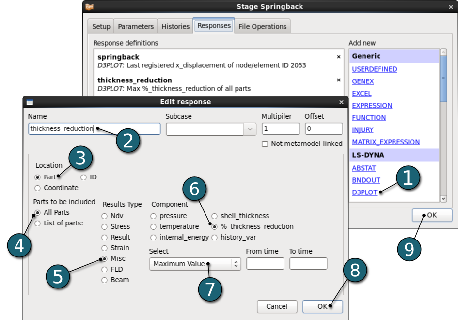
- Select D3PLOT as the type of response which is produced by LS-DYNA simulation.
- Enter thickness_reduction as the Name of the response.
- Select Part to specify the Location for the response.
- Select All Parts which are to be included in the response definition.
- As a Results Type select Misc. (Miscellaneous components).
- Select %_thickness_reduction as a Misc. Component.
- Select Maximum Value of the thickness reduction among all parts.
- Click on the OK button to end the response definition.
- Click on the OK button to proceed.
Home Screen Process Flowchart
- Double click on the Setup box for the conversion of parameters in input files to design variables of different types.
The Problem global setup dialog shall open.

Define Parameters
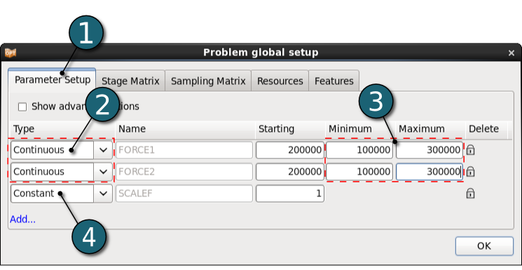
- Select the Parameter Setup tab.
- Select the variable Type of the first two parameters FORCE1 and FORCE2 as Continuous.
- Set the Minimum and Maximum Values of these continous parameters to 100000 and 300000, respectively.
- Select the Type of the parameter SCALEF as a Constant. By setting it as a constant, we conclude that SCALEF is not a design variable.
Stage Matrix
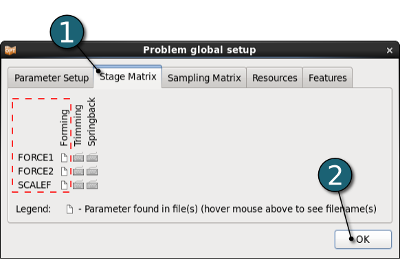
- Select the Stage Matrix tab.
- You find here a matrix of parameters vs. stages which provides an overview of the parameters defined in each stage.
- In this case the parameters are defined in the first stage - Forming.
- Hovering the mouse over a file icon shows a list of the files where the respective parameter is defined.
- Click on the OK button to proceed.
Home Screen Process Flowchart
- Double click on the Sampling Sampling box in order to define sampling settings and to import user-defined analysis results.
A Sampling Sampling dialog shall open.

Define Metamodel Settings
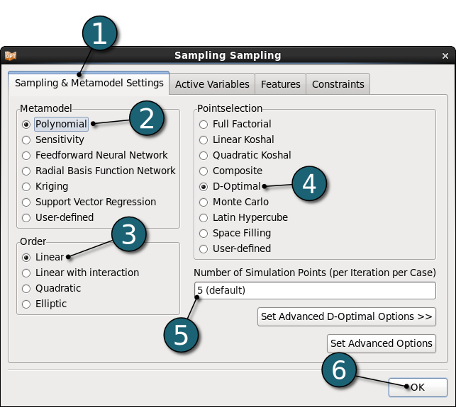
- Select Sampling & Metamodel Settings tab.
- Select Polynomial as the Metamodel type.
- Select Linear as the Order of the polynomial metamodel.
- Select D-Optimal for the Pointselection method.
- Use the default Number of Simulation Points, 5.
- Click on the OK button to proceed.
Home Screen Process Flowchart
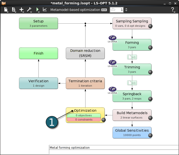
- Double click on the Optimization box to specify objectives and constraints for the design formulation and the optimization algorithm.
The Optimization dialog shall open.
Define Objective
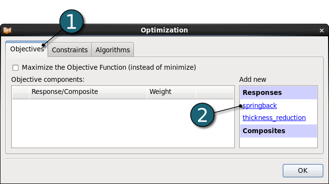
- Select the Objectives tab.
- From Responses list select spring_back as the objective.
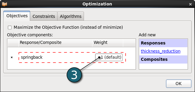
- Use the default Weight 1. If you have multiple objectives, you may assign different weights to each one according to their importance.
Define Constraints
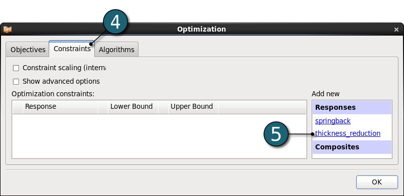
- Select the Constraints tab.
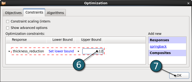
- Select thickness_reduction from the Responses list as the optimization constraint.
- Set the Upper Bound as 12.
- Click on the OK button to proceed.
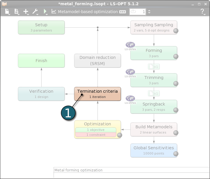
Depending on the optimization task and strategy, the user can specify tolerances on the design change, the objective function change or the accuracy of the metamodel. The user can also specify whether termination is reached if any one, or all of these criteria are met.
Home Screen Process Flowchart
- Double click on the Termination criteria box.
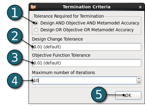
A Termination Criteria dialog will open.
Define Termination Criteria
- Select the Tolerance Required for Termination as Design AND Objective AND Metamodel Accuracy.
- Use the default Design Change Tolerance as 0.01.
- Use the default Objective Function Tolerance 0.01.
- Enter 10 for the Maximum number of iterations.
- Click on the OK button to proceed.
Home Screen Process Flowchart
Run LS-OPT
- Click on the Run button on the Control Bar.
- Click on Normal Run.
- The user can get information on the status of the current iteration during execution.
- For every stage the user has the option to observe the progress of the program execution by selecting the LED at the corner on the Stage box. It is possible to observe the Progress and View Log for more information about the execution process.
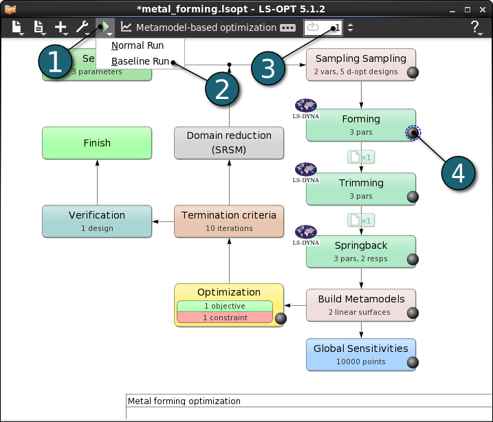
Home Screen Process Flowchart
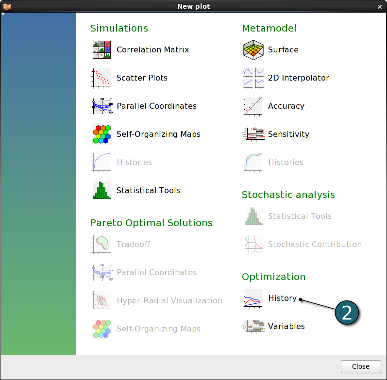
- Click on the Open the viewer icon in the control bar on the Home Screen Process Flowchart.
A New Plot window shall open.
- Choose History under the Optimization.
- The optimization history of a variable, dependent, response, constraint, objective, multi-objective or the approximation error parameters of pure responses (not composites or expressions) shows the changes of the respective values of the optimum over the iterations.

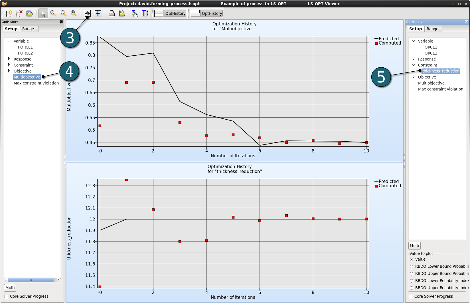
- Click on the Split vertical button to display two optimization histories together, i.e. the history of the objective springback and the constraint thickness_reduction.
- Select Multiobjective in the Setup dialog.
- Select the constraint thickness_reduction in the Setup dialog .
- In the plot below a black solid line indicates the predicted values for the objective and constraint. The red squares represent the computed values at the starting point of each iteration.
- For the constraints, the lower and upper bounds are displayed with a blue and red line, respectively.
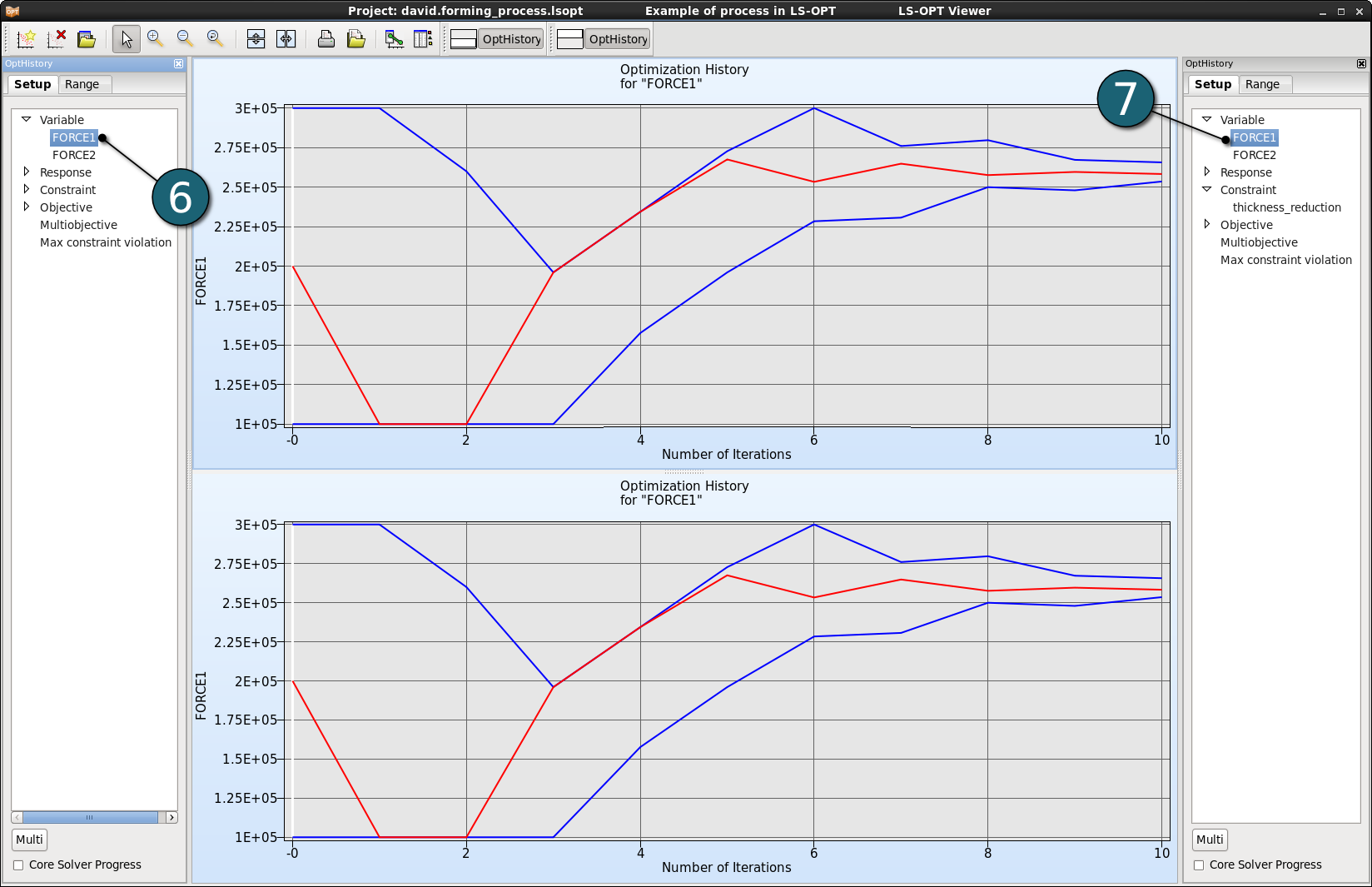
- Select FORCE1 under the Variable list in the Setup dialog to display the optimization history of this variable.
- Select FORCE2 under the Variable list in the Setup dialog to display the optimization history of this variable.
- The red line displays the variable value, the blue lines indicate the subregion bounds of the respective iteration.
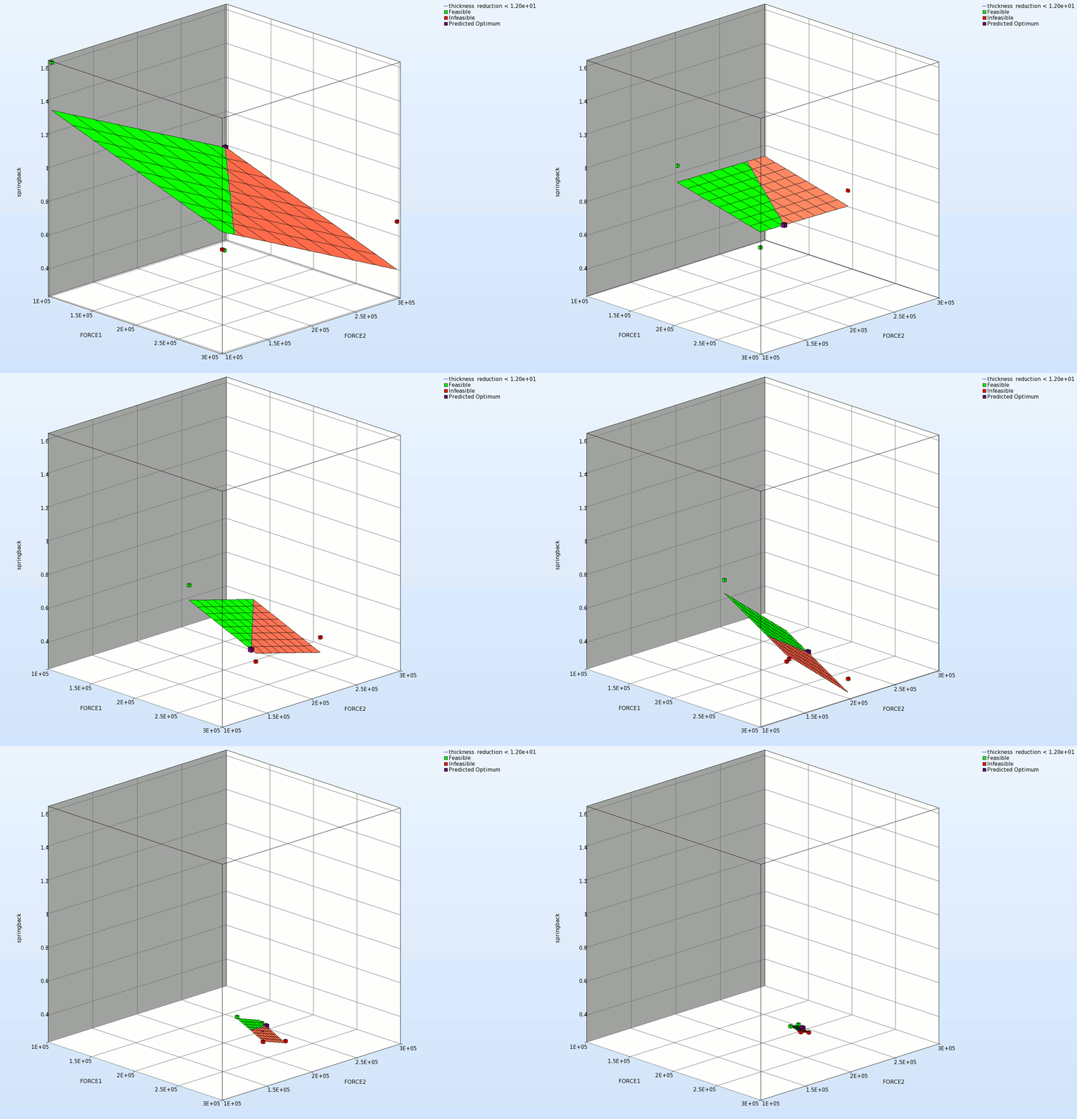
Two- or three-dimensional cross-sections of the metamodel surfaces and simulation points can be plotted and viewed from arbitrary angles.
New Plot - Surface
- Click on the New Plot button on the menu bar - ( or click on the View button on the Home Screen Process Flowchart as done in previous step for Scatter Plots).
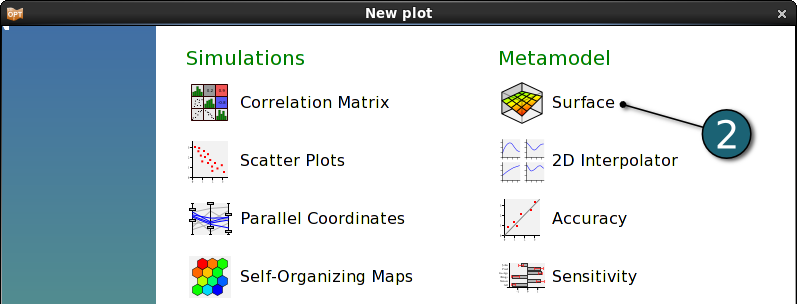
- Select under Metamodel the item Surface.

Plot Surface - Settings
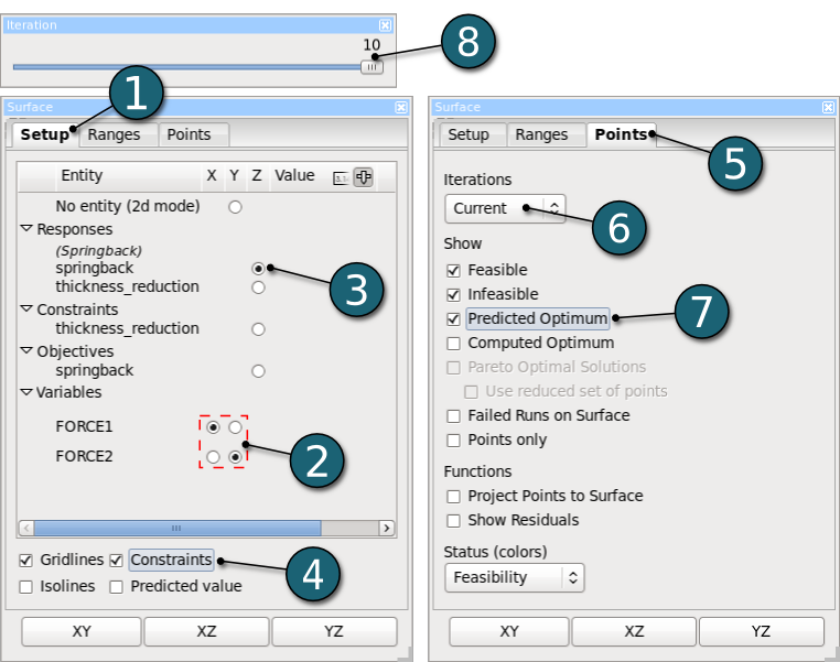
- Select the Setup panel.
- Set the variables FORCE1 and FORCE2 as x- and y-coordinate, respectively.
- Choose springback as z-coordinate.
- Select Constraints.
(Constraints are displayed on the surface.
Feasible regions are in green, the shade of red shows the degree of infeasibility (number of violated constraints), the colored line show the location where the constraints are exactly met.) - Go to the Points panel.
- Turn Iterations to Current.
- Show the Predicted Optimum point with all the feasible and infeasible points.
- Show the surface plot for the last Iteration 10.
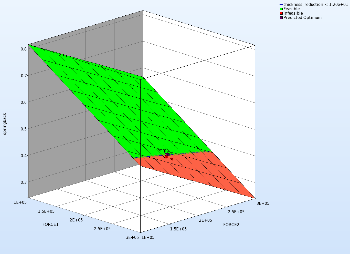
In the animated plot below we see the progress of the domain reduction method on the optimization process.
