Solution with LS-OPT https://www.lsoptsupport.com/examples/optimization/import-user-results/solution-with-ls-opt https://www.lsoptsupport.com/@@site-logo/LS-Opt-Support-Logo480x80.png

Solution with LS-OPT

Start-up
Task
Sampling
Setup
Stage
Composites
Optimization
Run
Results
Downloads

Working Directory and Extraction of necessary files

Create a working directory in the desired location to keep the LS-OPT project file and input files, as well as the LS-OPT program output, e.g. import_user_results.
Extract all the files required for this example from download section into the working directory.

Project Details

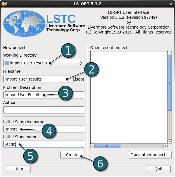
Select the Working Directory of the LS-OPT project.
Select a suitable name for the file under Filename (e.g. import_user_results). The extension .lsopt is appended automatically by LS-OPT.
Describe shortly the main optimization task under Problem Description (in this case, Import User Results, optional).
Choose a suitable name for the Initial Sampling (e.g. Import).
Choose a suitable name for the Initial Stage (e.g. Stage).
Click on the Create button to initiate the formation of the .lsopt file.

The main GUI window of LS-OPT opens.

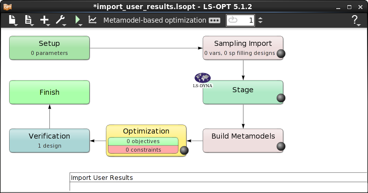
Home Screen Process Flowchart

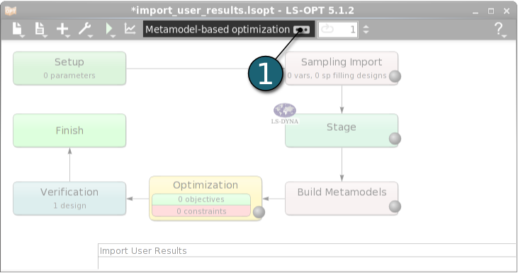
Click on the Show task settings icon to select the optimization task and strategy.

A window Task Selection shall open.

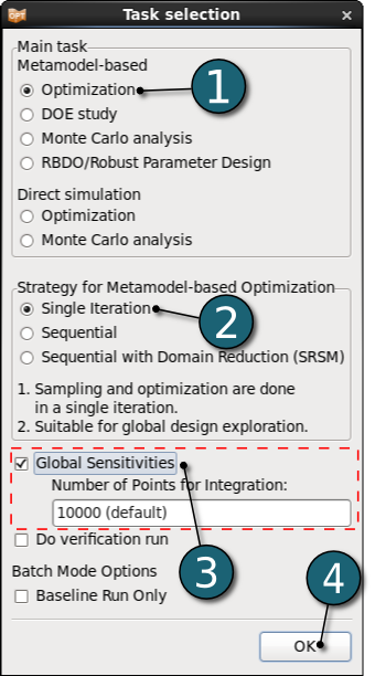
Define the Main Task

Select the radio button Optimization for the Matemodel-based main task.
Select the radio button Single Iteration for the Strategy for Metamodel-based Optimization. For imported results, this is the only strategy that makes sense.
In order to study Global Sensitivities on the metamodel check the adjacent box. The default number of sampling points for Monte-Carlo integration is 10000. Note that those points are evaluated on the metamodel, no simulations are necessary.
Click on the OK button to proceed.

After defining the main optimization task the Home Screen Process Flowchart takes the shape accordingly.

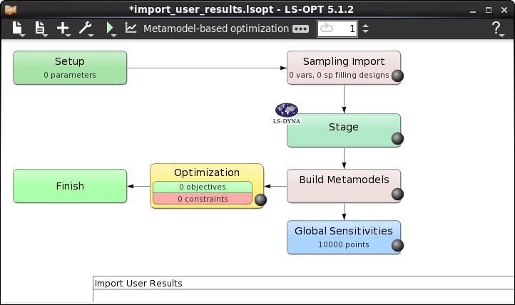
Home Screen Process Flowchart

Double click on the Sampling Import box in order to define sampling settings and to import the user-defined analysis results.

The Sampling dialog shall open.

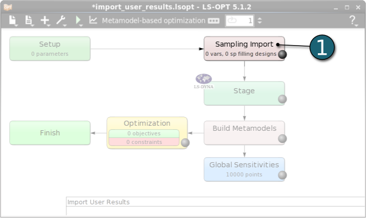
Import User Results

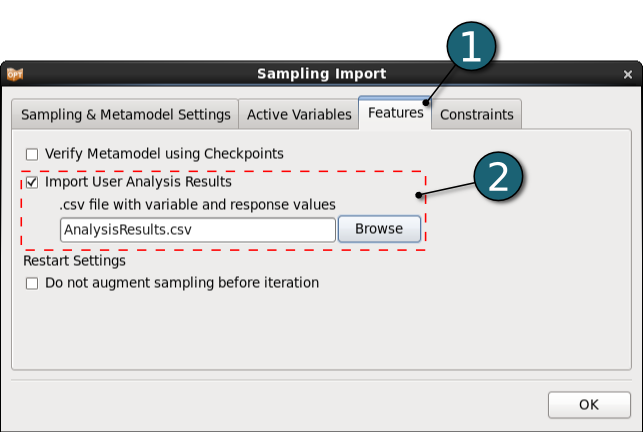
Select Features tab.
Browse for the file with the analysis results to be import, AnalysisResults.csv.

Define Metamodel Settings

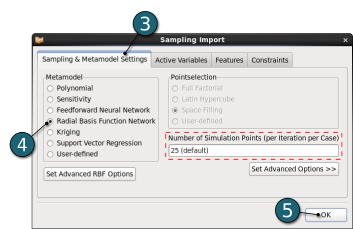
Select Sampling & Metamodel Settings tab.
Select Radial Basis Function Network as the Metamodel type.

The default number of Simulation Points is automatically imported from the results file - it is the number of points specified. If the user increases that number, a Point Selection scheme has to be chosen. In this case LS-OPT would augment the sampling points according to the selected point selection scheme and run additional simulations.

Click on the OK button to proceed.

Repair

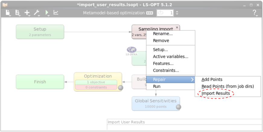
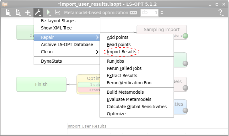
Now, the user results may be imported using Repair.

Repair can be run either from the right-mouse menu (top) of the Sampling box, or from the control bar Tools menu (bottom). This step converts the .csv format to the LS-OPT database format ready for analysis.

Build Metamodels

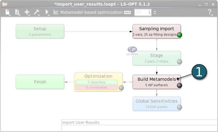
Double click on the Build Metamodels to see that the Build Metamodels box is coupled to the same dialog as the Sampling box. It is displayed at the end of the process to correctly represent the optimization process.

Home Screen Process Flowchart

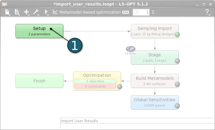
Double click on the Setup box.

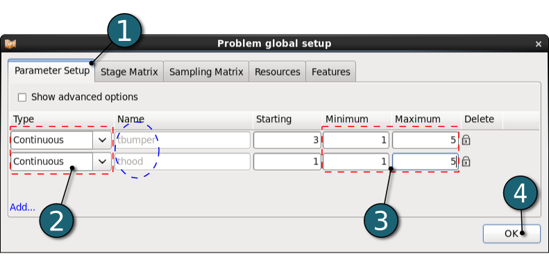
The Problem global setup dialog shall open.

Define the Variables

Select the Parameter Setup tab.

The variable names, values and ranges are read from the .csv file to be imported.

Select the variable Types as Continuous.
Adjust the variable bounds to 1 for Minimum and to 5 for Maximum for both variables.
Click on the OK button to proceed.

Home Screen Process Flowchart

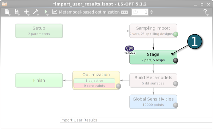
Double click on the Stage box.

The Stage dialog shall open.

Since we have user anaylsis results for the optimization and don't want to run additional simulations, we don't need to define a solver command and inputfile, respectively.

In this case we skip the Stage - Setup step.

Responses for Optimization

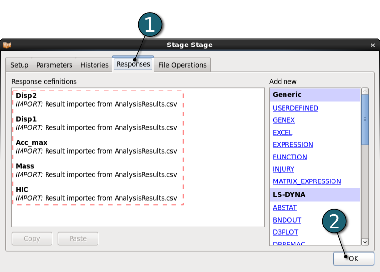
Select the Responses tab.

The responses defined in the imported file are displayed here.

Click on the OK button to proceed.

Home Screen Process Flowchart

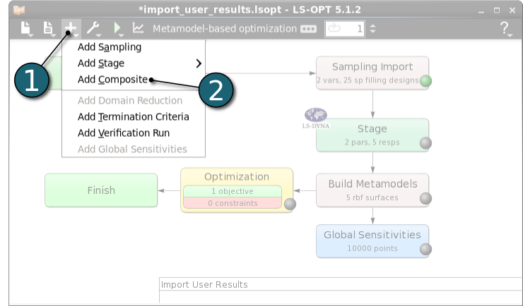
Click on the Add menu in the Control bar.
Select Add Composite.

The Composites dialog shall open.

Define Composites

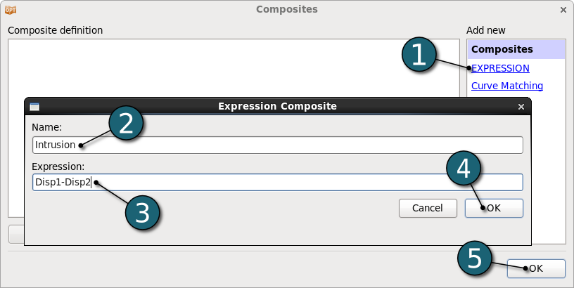
Select Expression as a composite type which presents a mathematical expression using previously defined (imported) responses.
Enter Intrusion as a Composite Name.
Enter Disp1-Disp2 as the Expression.
Click on the OK button to end the definition of the composite expression.
Click on the OK button to proceed.

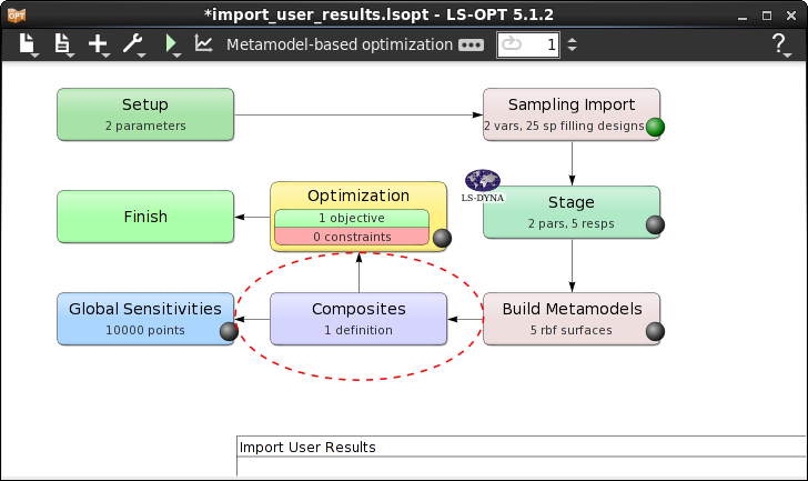
After defining the composite expression the Composites box takes its place in the Home Screen Process Flowchart.

Objectives
Constraints

Specification of objectives and constraints for the design formulation.

Home Screen Process Flowchart

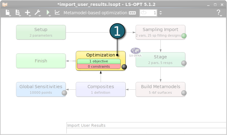
Double click on the Optimization box.

The Optimization dialog shall open.

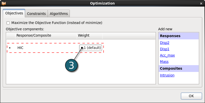
Define Objective

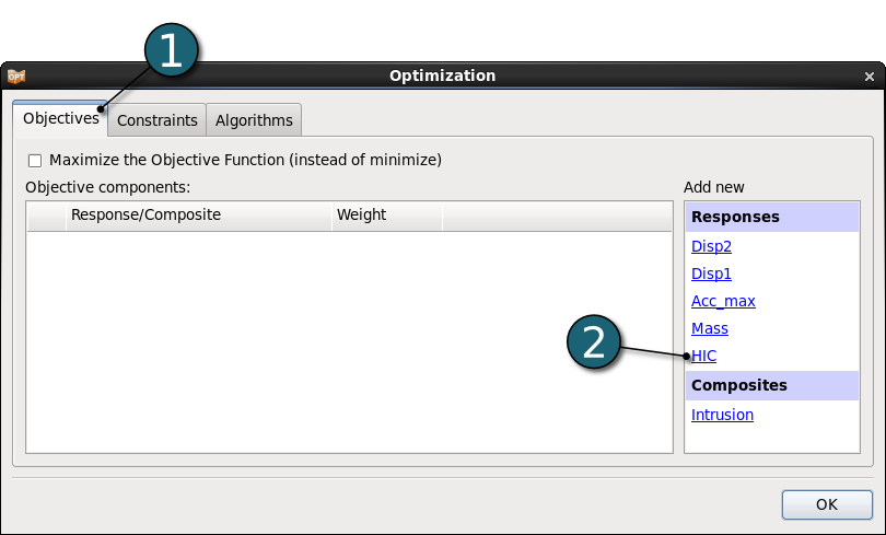
Select the Objectives tab.
From Responses list select HIC as the objective function.
Use the default Weight 1. If you have multiple objectives, you may assign different weights to each one according to their importance.

Define Constraints

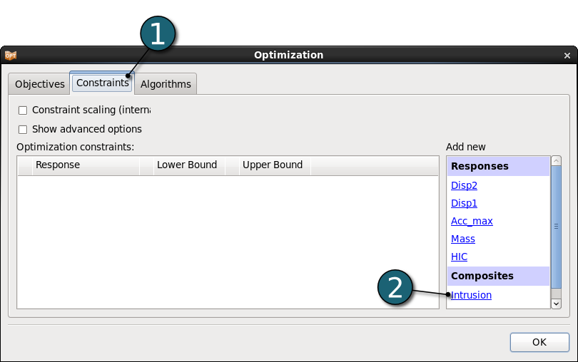
Select the Constraints tab.
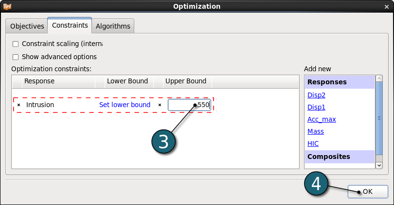
Select Intrusion from the Composites list as the optimization constraint.
Set the Upper Bound as 550.
Click on the OK button to proceed.

Home Screen Process Flowchart

Run LS-OPT

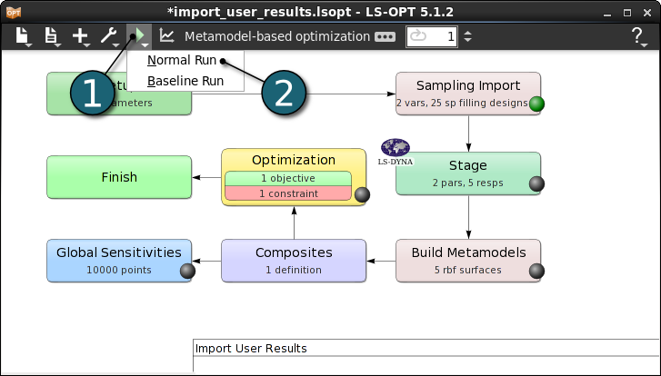
Click on the Run menu in the Control Bar.
Select Normal Run for execution.

Surface
Accuracy
Sensitivity

Two- or three-dimensional cross-sections of the metamodel surfaces and simulation points can be plotted and viewed from arbitrary angles.

Surface Plot

Click on the Open the viewer button in the control bar on the Home Screen Process Flowchart.
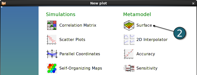
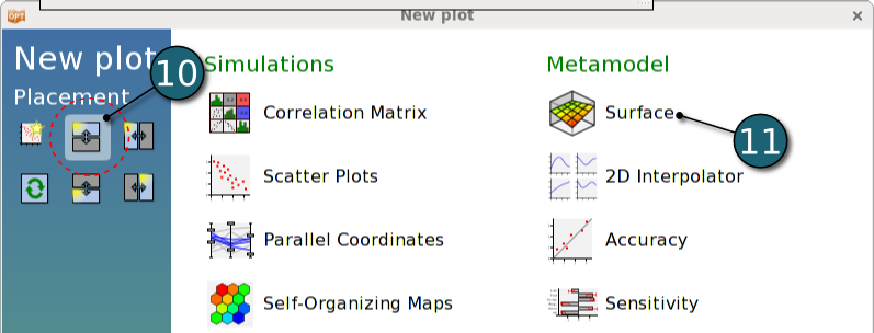
Choose Surface plot under Metamodel from the New plot window.

Surface Plot Options

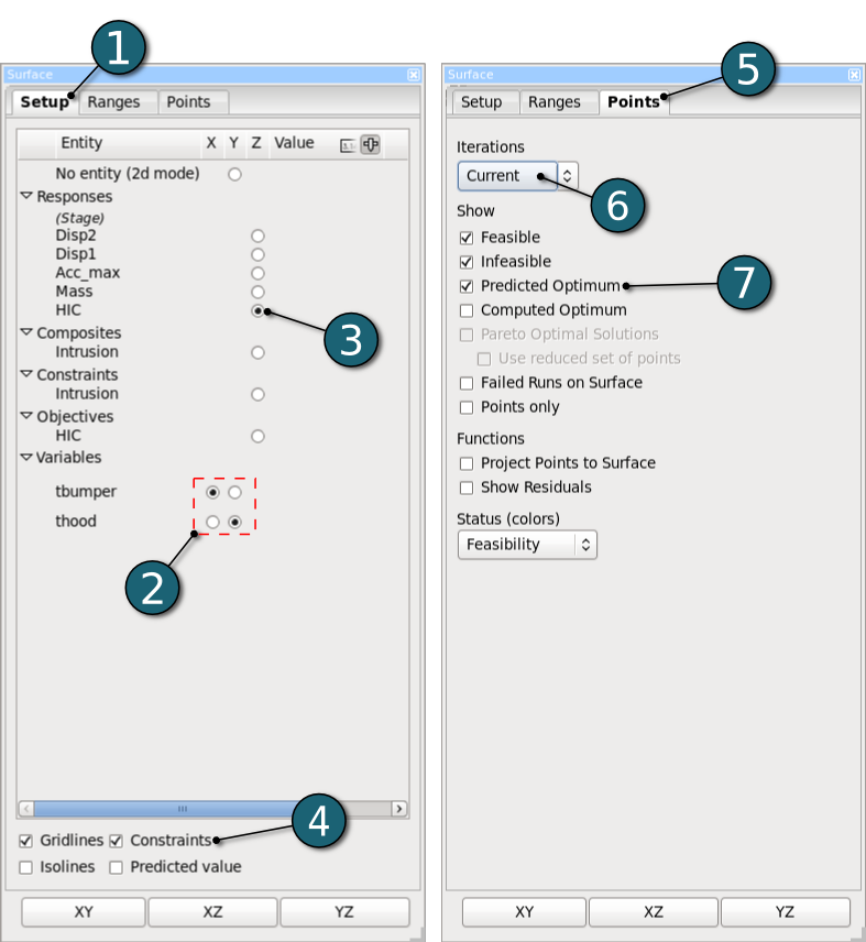
Select Setup tab.
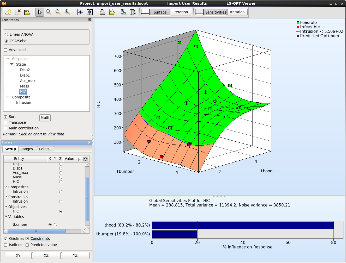
Select the design variables tbumper and thood as the x and y entities, respectively.
Select HIC response as the z entity.
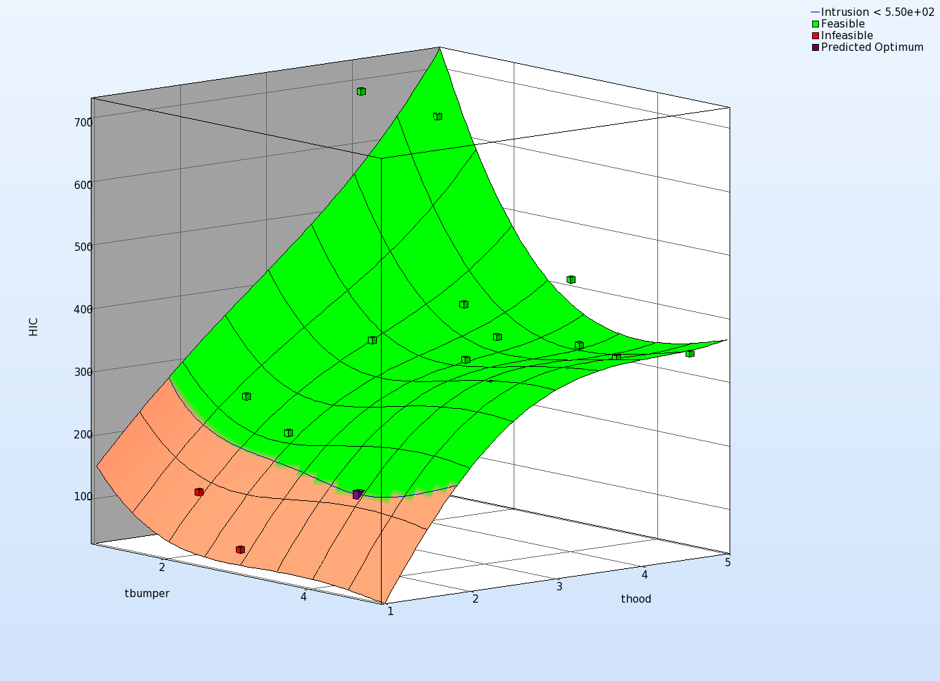
Select Constraints to be shown on the plot. Constraints are displayed on the surface. Feasible regions are green, the shade of red shows the degree of infeasibility (number of violated constraints), the colored lines show the location where the constraints are exactly met.
Select Points tab.
Select Current Iteration points to be shown on the surface plot.
Show the Predicted Optimum point.

In the Surface plot we see that the Optimum point locates on the minimum of the feasible area.

The accuracy of the metamodel fit for the selected response or composite is illustrated in this section.

Accuracy Plot

Click on the New Plot button in the menu bar -(or click on the Open the viewer button on the Home Screen Process Flowchart as done in previous step for Surface plot.)
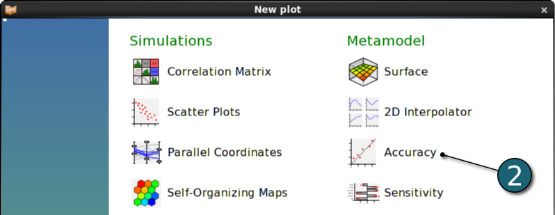
Select Accuracy under Metamodel.
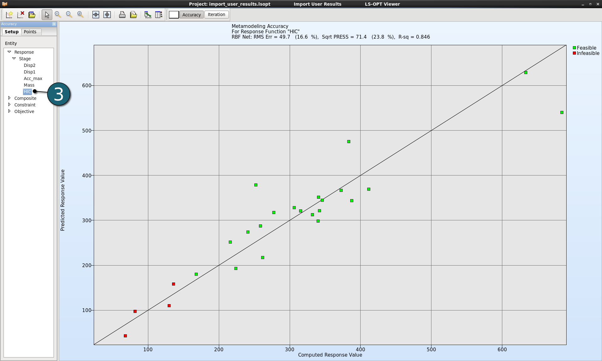
Select HIC response from Accuracy option dialog to display its accuracy.

The Accury plot displays the computed values (in this case from the .csv file) vs. the predicted values evaluated on the metamodel. The closer the points are to the black line, the better the metamodel fits the points.The error measures displayed in the title of the Accury plot may also be used to judge on the quality of the metamodel.

In this example we will observe the Global Sensitivity Analysis (GSA/Sobol) results.

Sensitivity Plot

Click on the New Plot button in the menu bar - (or click on the Open the viewer button on the Home Screen Process Flowchart as done for the first Surface plot step.)
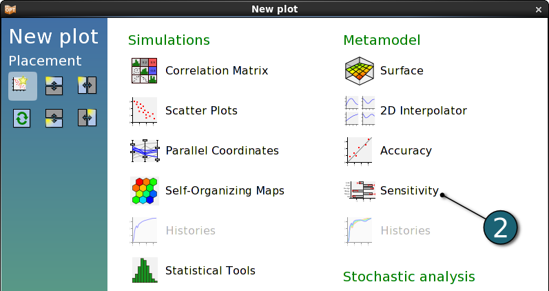
Select Sensitivity under Metamodel from the New plot window.
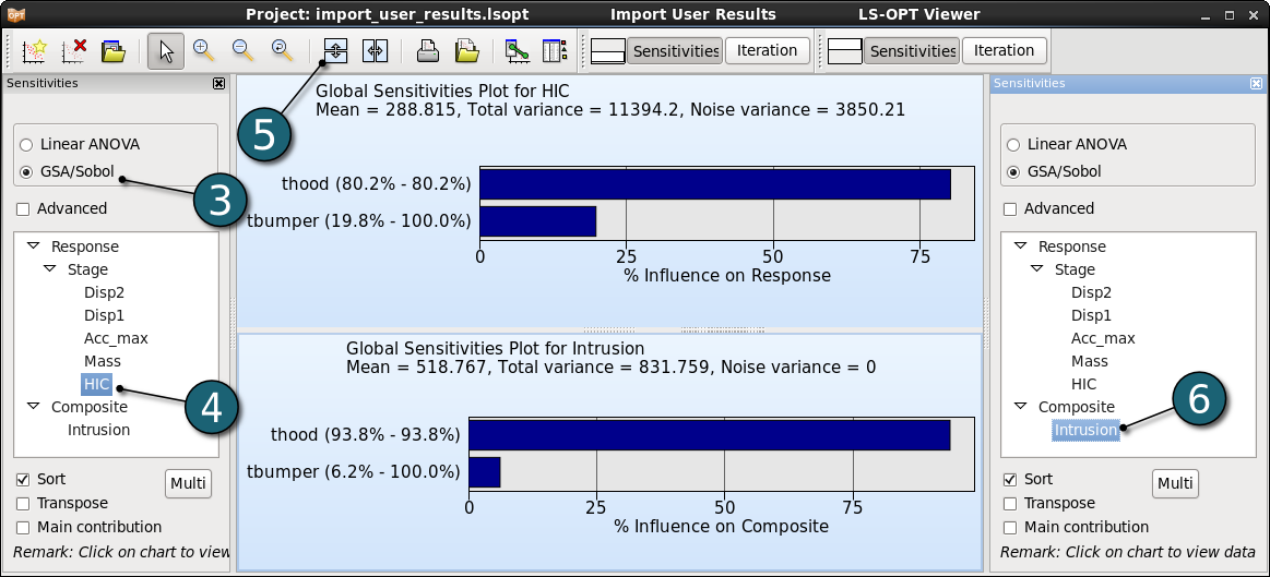
Select GSA/Sobol from the Sensitivities options dialog.
Select HIC response.
Click on the Split vertical button to have a second Sensitivity plot in the same window.
Select Intrusion from the Sensitivities options dialog of the second plot.

On the plot below we see that the design variable thood has clearly much more influence than tbumper on both the response HIC and constraint Intrusion.

Select one of the plots and then click on the Delete plot icon.
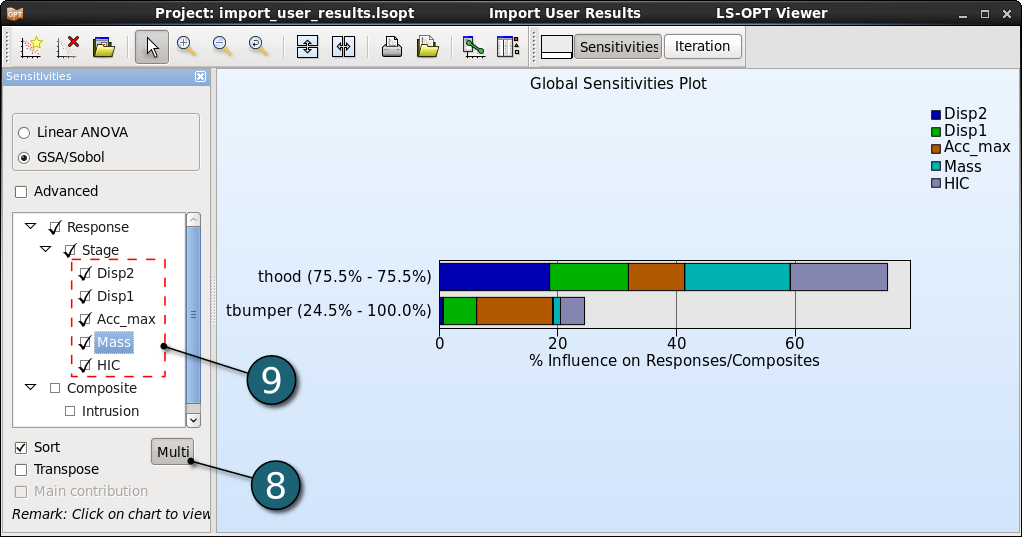
Select the Multi option.
Select all Responses to find the most sensitive variable on the full problem.

On the plot on the right side we can see the influence of each design variable on each response of the system. thood has the most influence on that load case.

In order to have different types of plots in the same window we have to choose Split vertically option in the New Plot window.
Select Surface plot and set the same options as in the previous Surface plot step.

The Surface plot can now be used to confirm the GSA results.

Download:	for Linux & Windows
	import.tgz (1.9 kB)