ANSA Opt. Task
Defining the Optimization Task
In this step will be defined the pre-processing sequence that will be connected to LS-OPT. This sequence of actions will be invoked in every optimization loop and every action of it will be executed in the defined order modifying the shape and parameters of the model. All these actions take place before the run of the solver.
When the sequence runs the following tasks are executed:
- Reading Design Variable values from an ASCII file
- Modify the model according to the values of the ASCII file
- Output the model in LS-DYNA format
In order to skip the previous sections the user can use the rail_morph.ansa file where the morphing actions are already defined. However there is the need to rename the file as rail.ansa.
|
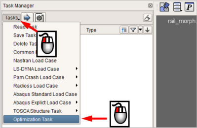
The optimization sequence will be defined through the Task Manager Tool. This sequence will be saved in the ANSA database when the user saves the database. Use the |
|
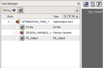
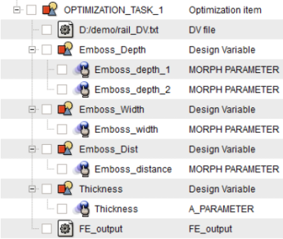
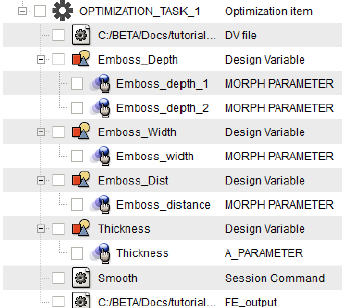
A default Optimization Task is defined which contains the following Task Items:
At this time the Optimization Task is at Definition mode. In this mode the user is able to define and modify the Task. This is the default mode when an Optimization Task is created. To run the Optimization Task the user should switch to the Execution mode. This action is defined in a later section. |
|
|
Design Variables for Morphing Parameters
The first Design Variable will control the depth of the embosses. To achieve this, the Design Variable will control the Morphing Parameters Emboss_depth_1 and Emboss_depth_2.
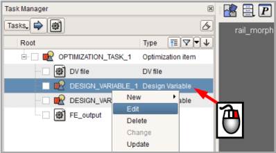
Right click to the Design Variable Item and select the Edit function to define the type and boundaries of the design variable.
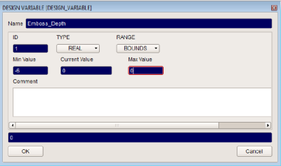
In the window that appears set the TYPE pull-down to REAL and the RANGE to BOUNDS. With these settings the Design Variable can get any real value between the Min and Max Value. Enter the values:
- Min Value : -6
- Current Value : 0
- Max Value : 0
Optionally enter a new name for the design variable (Emboss_Depth).
Pick OK to accept the settings.
NOTE : ALWAYS USE NAMES FOR THE DESIGN VARIABLES WITH NO SPACES IN ORDER TO PROPERLY READ IN LS-OPT.
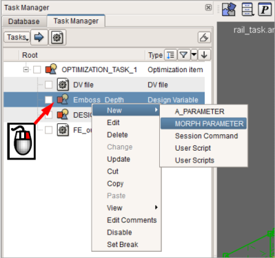
Right click on the Design Variable Item and select the New>MORPH PARAMETER. A new Task Item of type MORPH PARAMETER is created and it is connected with the Emboss_Depth design variable.
- Right click on the MORPH PARAMETER Task Item and select Edit.
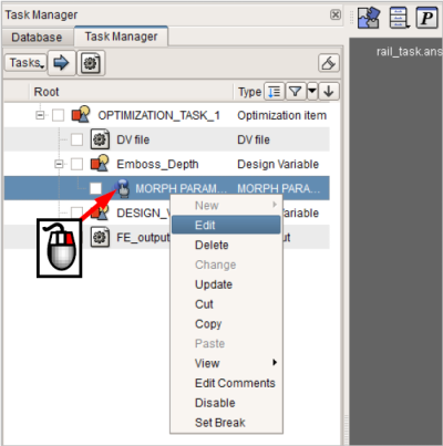
A window containing the already defined Morphing Parameters from the Morphing Tool appears. Select the first Morphing Parameter and pick OK to confirm. Now the MORPH PARAMETER Task Item is associated with the Emboss_depth_1 Morphing Parameter. The Item’s name is modified accordingly.
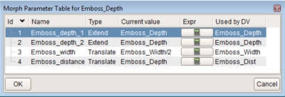
In the same way create one more MORPH PARAMETER Task Item under the same design variable. Select the second Morphing Parameter and confirm.
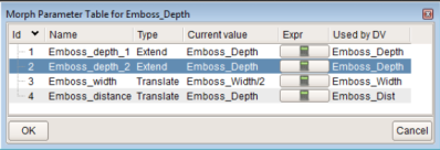
The first design variable is ready. Two Morphing Parameters are associated to this design variable since, to modify the depth of the embosses, two Morphing Parameters are needed. During the run of the optimization sequence the current value of the Design Variable will be applied to the associated Morphing Parameters and the model will be morphed accordingly.
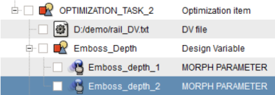
Design Variable for the Emboss Width
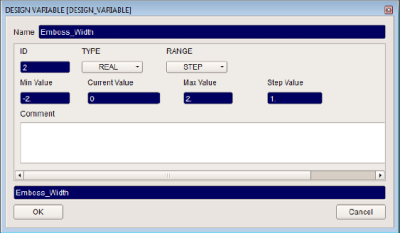
Right click on the second Design Variable Item and select the Edit to open the design variable card. Switch the TYPE pull-down to REAL and the RANGE to STEP. With these settings the Design Variable can get the real values between the Min and Max Value by a specified step. Enter the values:
- Min Value : -2
- Current Value : 0
- Max Value : 2
- Step Value : 1
Optionally enter a new name for the design variable (Emboss_Width) and press OK to accept the settings.
Right click on the Design Variable Item and select the New>MORPH PARAMETER. A new Task Item of type MORPH PARAMETER is created and it is connected with the Emboss_Width Design Variable.
Right click on the new MORPH PARAMETER Task Item and select Edit.
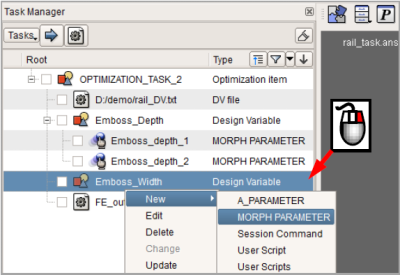
In the window that appears select the third Morphing Parameter and press OK.
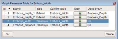
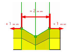
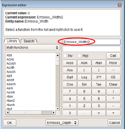
The way that the Emboss_width Morphing Parameter has been defined leads to the following result: Morphing the above parameter by 1 mm moves both edges of the emboss to the opposite sides resulting to a movement of 2 mm. To overcome this problem a calculation can be added between the Design Variable and the Morphing Parameter.
Click on the Calculator symbol of the relative parameter.
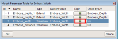
The current value is displayed which is the Parameter's name. Type /2 to divide by two, the current value. Press ENTER to accept the calculation entry. Pick OK to confirm and exit the window.
Design Variable for the Emboss Distance
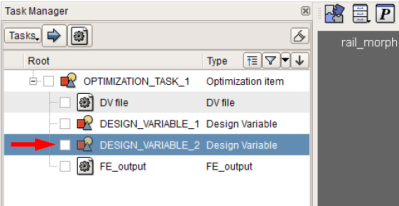
The third design variable will control the distance between the embosses. Create a new Design Variable Task Item and Edit it. Leave the TYPE pull-down to REAL and the RANGE to BOUNDS. Enter the values:
- Min Value : -5
- Current Value : 0
- Max Value : 10
Optionally enter a new name for the design variable (Emboss_Dist) and press OK to accept the settings.
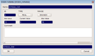
Right click on the Design Variable Item and select the New>MORPH PARAMETER to create such Task Item.
Right click on the new MORPH PARAMETER Task Item and select Edit.
In the window that appears select the fourth Morphing Parameter and press OK to confirm.

The Design Variable that controls the emboss distance is ready.
Design Variable for the Thickness
Define one more Design Variable Task Item. This Design Variable will control the shell thickness of the model.
Right click on this Design Variable Item and select the Edit to open the design variable card. Switch the TYPE pull-down to REAL and the RANGE to LIST. With these settings the Design Variable can get the real values from a list since the shell thickness can only have discrete values. Enter the values:
Text Values : 0.8, 0.9, 1, 1.2, 1.4, 1.7
Current Value : 1.2
Optionally enter a new name for the Design Variable (Thickness) and press OK to accept the settings.
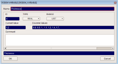
Right click on the Design Variable Item and select the New>A_PARAMETER. A new Task Item of type ANSA Parameter is created and it is connected with the Thickness design variable.
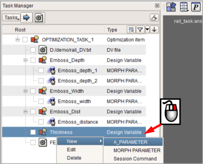
Right click on the new A_PARAMETER Task Item and select Edit.
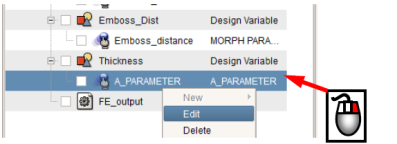
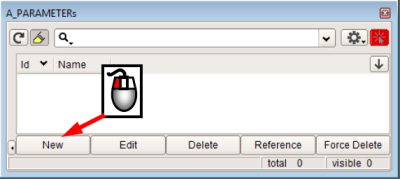
The A_PARAMETERs window opens. Pick the NEW button to define a new ANSA Parameter.
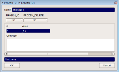
The card of the new ANSA Parameter opens. Enter a name (e.g. Thickness) and a valid value for the shell thickness. In this case valid is a value not equal to zero. Press OK to confirm.
As the Parameter is defined double click on it to assign it to the A_PARAMETER Task Item.
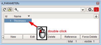
Now the ANSA Parameter is assigned to the relative design variable. To be able to control the shell thickness of the model the parameter should substitute the thickness value in the property card.

Open the property list using the button of the Containers toolbar menu, select the property of the rail body and pick Edit.
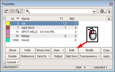
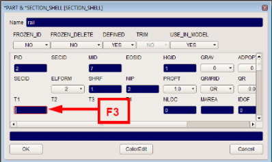
The SECTION_SHELL card opens. Delete the content of the field T1 and pick the F3 key. F3 Key is enabling the usage of ANSA Parameters in the relative field.
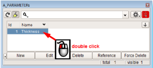
The A_PARAMETERs list opens. Select the Thickness ANSA Parameter by double click on it.
The expression “= Thickness” is entered in the T1 field. Now the shell thickness of the specific property will be controlled by the Thickness ANSA Parameter and subsequently by the relative design variable.
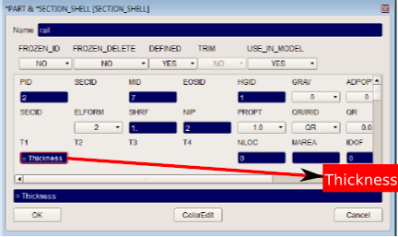
The design variable which controls the shell thickness of the model is ready.
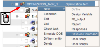
Session Commands can be added to the optimization sequence to apply a specific operation. The session commands can be added under a Design Variable Task Item or at the main root of the Optimization Task. In this example a session command will be added to the main root which will smooth the mesh of the model after the shape modification.
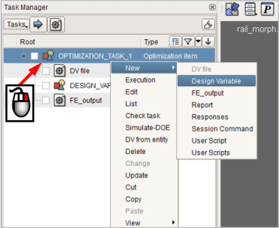
Right click on the Optimization Task and select New>Session Command in the pull-down menu that appears.
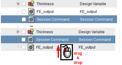
A new Task Item is defined at the end of the Optimization Task.
Drag and drop the new Task Item one step above since this command should be executed before the final output of the FE model.
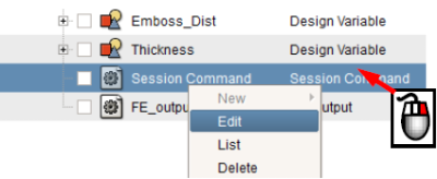
Right click on the Session Command Item and select Edit from the pull-down menu.
In the window that appears are listed all the available session commands. Select the command “MESH>SHELL MESH>SMOOTH:” and press ENTER to confirm.
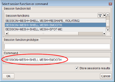
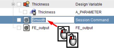
Optionally change the name of the Task Item. To do this, select it with left button and then single click on it.
The Smooth command will be executed after the morphing of the model and the change of the thickness according to the defined Design Variables.
Design Variables File
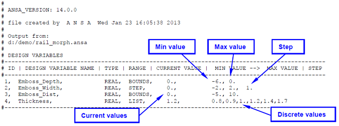
The DV Input file is an ascii file which contains all the data contained in every design variable card. Through this file, the Optimization Task of ANSA is connected to the optimizer. This file can be created with the functionality of the Optimization Task. When ANSA will be connected to the optimizer the file will be used as input file for the design variable values. The optimizer will change the Current Values of each design variable in this file. In every optimization loop these values will update the Current Values of the Design Variables.
Every action that is defined under any Design Variable Task will be executed using these values.
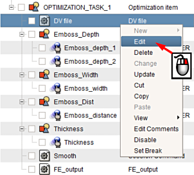
Right click on the DV File Item and select Edit from the pull-down menu.
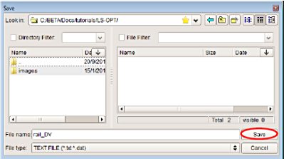
In the file manager that appears enter the path where the DV File should be saved. It is recommended to save the file to the working directory.
NOTE: Even if the input file is defined with an absolute path, LS-OPT will overwrite this path since in every iteration a new directory will be created containing all the data of the experiment.
The DV File Task is defined. However the file is not yet created and saved. The file will be saved as soon as the user switches from Definition to Execution mode.

The DV File is shown below.
FE Output File
A last Task Item is used to create an output of the model in FE format.
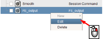
Right click on the FE-output Task Item and select the Edit function.
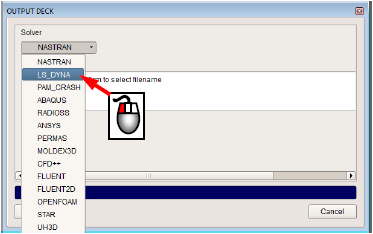
The OUTPUT DECK window appears. Select the LS_DYNA option from the pull-down to output the model in this format. Press OK to confirm.
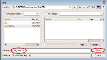
The file manager window opens. Select the filename for the output file and confirm. In this example the name of the file is rail.key.
NOTE: Make sure to specify the file without a path!
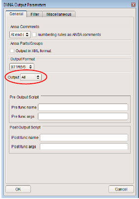
The DYNA Output Parameters window opens. Select the options for the LS-DYNA file and confirm. In this example the user could use the “All” option to output the whole model.
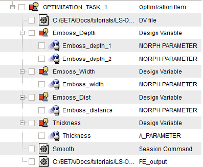
The FE Output Task Item is defined.
However, the file is not yet created and saved. The file will be created when the Optimization Task runs in the Execution mode.
Before connect the optimization sequence with LS-OPT the user is able to simulate the actions that will take place in each loop and check the results.
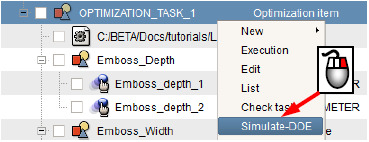
Right click on the Optimization Task and select the Simulate-DOE function.
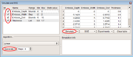
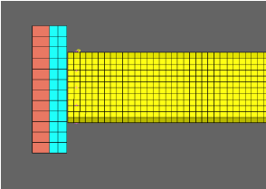
The Simulate and DOE window opens displaying all the defined Design Variables.
- To simulate the shaping according to the design variable values, ensure that the relative Design Variables are activated.
- Pick the Generate button to generate teh defined number of states. The relative combinations are created in the Table.
- Pick the Simulate button. The animation buttons become active.
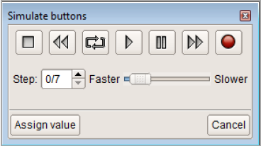
- Use the activate buttons (play, stop, forward, etc..) to animate the model though the design variable values. Alternatively use the Current step slide bar to go to a specific step. The Frame rate slide bar will change the animation speed.
- After checking the model validity for any combination of design variable values pick the Esc to quit. The model returns to its initial state.
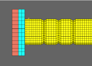
NOTE: The actions that cannot be restored (for example Smoothing) are excluded from the simulate action.
Run the Optimization Task
After the definition and the checking the model for different design variables combinations, the ANSA file should be saved with the Optimization Task in Execution mode.
Right click on the Optimization Task and select Execution.
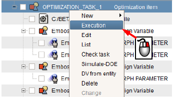
At this time the DV File is created. In case that the DV File already exists a warning window appears. Pick OK to overwrite the DV File.
NOTES: If the Cancel button is selected, the Optimization Task will remain in Definition mode. This ensures that the Optimization Run won't run using a not compatible DV File.

The Optimization Task is able to switch to Execution mode only if all Task Items are defined properly.
The symbol of the Optimization Task indicates that the current mode is the Execution.
Now, save the ANSA file. The model is ready to be connected to LS-OPT.
The complete data set (input and command files) is available for download:
For Linux
For Windows

