LS-OPT
Working Directory and Extraction of necessary files
- Create a working directory in the desired location, e.g. RAIL.
- Extract all the files for the RAIL from download section into the working directory.
Project Details
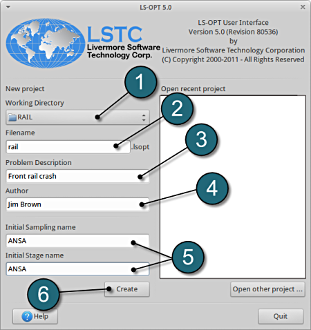
- Select the Working Directory of the LS-OPT project.
- Select a suitable name for the file under Filename (e.g. rail). The extension .lsopt is appended by LS-OPT.
- Description of the main task can e.g. be a suitable name for Problem Description ( in this case, Front rail crash, optional) .
- Input the name of the Author (optional).
- Choose a suitable name under the Initial Sampling name and Initial Stage name (e.g. ANSA).
- Press the Create button to initiate the formation of the input file.
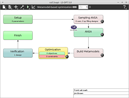
- The main GUI window of LS-OPT opens.
Home Screen Process Flowchart
-
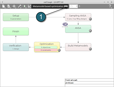
Select the Task icon.
A window Task selection shall open.
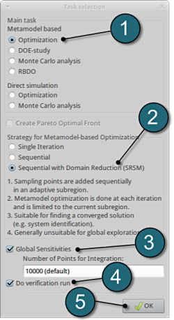
Define the Main Task
- Select the radio button Optimization for the selection of the main task.
- The selection of the strategy is made to Sequential with Domain Reduction (SRSM). The optimization is performed in an iterative process then.
- To study the Global Sensitivities for the input parameters remember to select the adjacent radio button.
- The user has a choice to Do verification run by selecting the option.
- Push the OK button to proceed.
In this step the coupling of ANSA with LS-OPT will be demonstrated.
Home Screen Process Flowchart
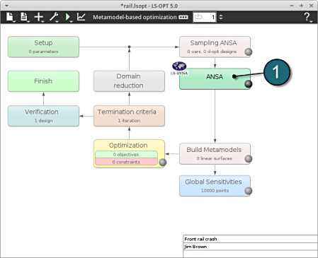
- Select the ANSA box.
A window Stage ANSA shall open.
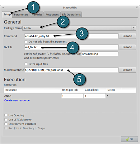
Define Pre-Processor
- Select the Setup tab.
- As Package Name select ANSA.
- Browse for the Command that runs ANSA (in this case ansa64, add the comand line option -lm_retry 60 to avoid that the optimization stops because of missing ANSA licenses ). Make sure to use ANSA v.14.x or later if you use the files provided.
- Browse for the DV File of the design variables: rail_DV.txt.
- Browse the Model Database rail_task.ansa, for this example. The path of the selected file is displayed on the screen.
In order to skip the previous steps the user can use the provided rail_DV.txt and rail_task.ansa file where the morphing actions and the Optimization Task are already defined. Make sure that the Optimization task is set to Execution mode in ANSA before running the optimization. Otherwise the files generated by following the steps described in ANSA Morph and ANSA Opt. Task may be used.
!NOTE: Open weblinks in New Tab for reference.
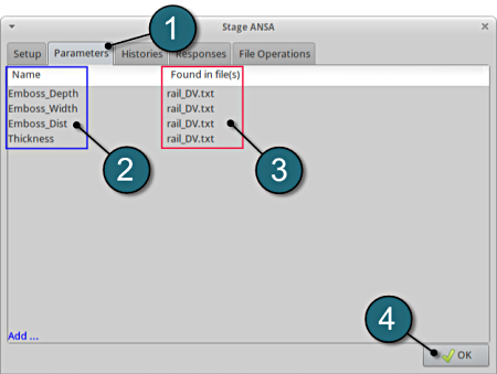
The parameters located in the selected DV File can be visualized in the adjoining tab Parameters.
Design Parameters.
- Select the Parameters tab.
- The Names of the various design parameters are listed here.
- The created variables are read in from the file rail_DV.txt.
- Select OK to proceed.
The DV File rail_DV.txt is shown below for reference.
# DESIGN VARIABLES
#-----------------------------------------------------------------------------------
# ID | DESIGN VARIABLE NAME | TYPE | RANGE| CURRENT VALUE|MIN VALUE-->MAX VALUE|STEP
#-----------------------------------------------------------------------------------
 1,  Emboss_Depth,  REAL,     BOUNDS,    0., -6., 0.
 2,  Emboss_Width,  REAL,     STEP,      0., -2., 2.,  1.
 3,  Emboss_Dist,  REAL,     BOUNDS,    0., -5., 10.
 4,  Thickness,  REAL,     LIST,    1.2,0.8,0.9,1.,1.1,1.2,1.4,1.7
#-----------------------------------------------------------------------------------
Home Screen Process Flowchart
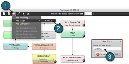
- To add a new Stage select the Add (denoted as +) at the task bar of the GUI.
- Select the Add Stage > in ANSA option.
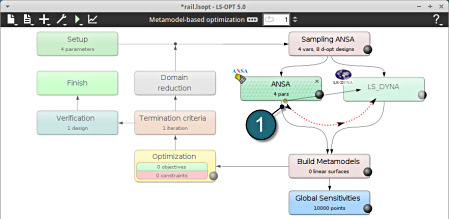
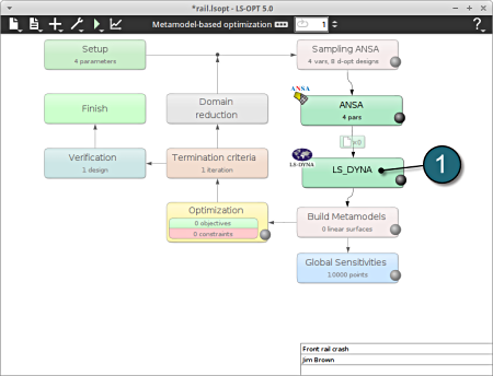
- Select a suitable name for the new stage e.g. LS_DYNA and press OK . The main LS-OPT GUI includes a new Stage LS_DYNA (see image below).
Dependencies of Stages
- The dependency of the stages is set by dragging the arrow head from the stage ANSA to the stage LS_DYNA.
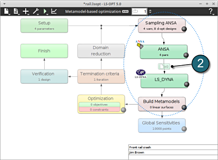
The figure below illustrates the re-positioning of the new Stage LS_DYNA in the LS-OPT process flow. The stage boxed can be moved using the left mouse button to display the process chain as desired. There is also an automated option to layout the stage boxes in the Tools menu.
- Since the ANSA output file is used as LS_DYNA input file, the definition of a File Transfer is necessary. Select the respective icon.
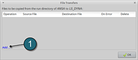
A window File Transfers shall open.
File Transfers
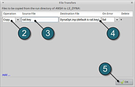
- Select the Add.. button.
- For Operations, choose Copy.
- Enter the name of the Source File to copy from the ANSA directory to LS-DYNA. In this case enter rail.key.
- Enter the name of the Destination File to be copied to LS-DYNA. In this case enter DynaOpt.inp.
- Select OK to continue.
Now, the user can define the properties of the LS-DYNA Stage.
Home Screen Process Flowchart
- Select the LS_DYNA box.
A window Stage LS_DYNA shall open.
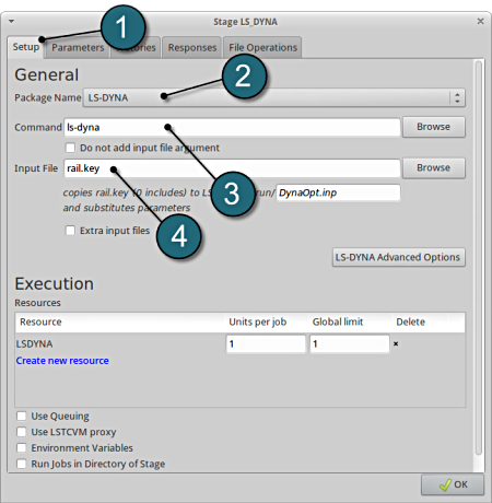
Define Input File Name and Command
- Select the Setup tab.
- Select the Package Name for the stage to LS-DYNA.
- For Command specify the LS-DYNA executable ls-dyna (This name can be different on your computer). On Windows, the command has to be specified using the absolute path.
- For Input File enter rail.key. This file is generated by the upstream stage ANSA.
Responses for Optimization
- The various responses for the optimization problem can be added by the following steps:
Add First Response
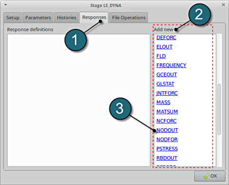
- Select the Responses tab.
- Select the suitable response type from the various option available from the list under Add new.
- For the first response select the option NODOUT , which represents an interface to LS-DYNA nodout results. Note that LS-OPT reads the results from the binout database.
A separate window emerges named; New response. This enables the user to define the response in suitable steps.
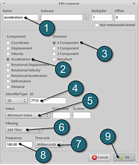
Define x-acceleration of node 7710
- For Response name enter acceleration.
- For Component select from the list Acceleration.
- For Direction select X Component.
- For node ID enter 7710.
- Select the Minimum Value option under Select. This will choose the max. value of acceleration in x-direction during the crash.
- For Filtering choose SAE Filter.
- Select Milliseconds as the Time unit.
- Enter 180.0 for Frequency.
- Select the OK button to add the response.
- The New response dialog closes and returns to the main page of the Responses tab in the Stage LS-DYNA window.
NOTE: In this case, the magnitude of acceleration is negetaive, hence its necessary to measure the minimum value.
Add Second Response
- To add an additional response select the option NODOUT from the Add new list on the Responses tab.
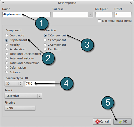
Define x-displacement of node 7710
- For Response name enter displacement.
- For Component select from the list Displacement.
- For Direction select X Component.
- For node ID enter 7710.
- Select the OK button to add the response.
- The New response dialog closes and returns to the main page of the Responses tab in the Stage LS-DYNA window.
Add Third Response
- To add an additional response select the option Mass from the Add new list on the Responses tab.
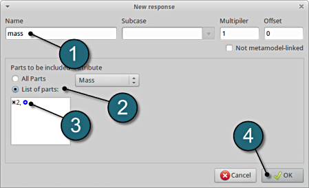
Define mass responses for structural component
- For Response name enter mass.
- For Parts to be included select List of parts.
- In the empty box underneath enter 2.
- The part ID numbers can be found in the main page of the problem description.
- Select the OK button to add the response.
- The New response tab closes and returns to the main page of the Responses tab in the Stage LS-DYNA window.
Responses Review
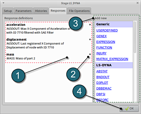
- The defined responses can be reviewed in the tab of the Responses under the Response definitions. Necessary changes can be made by selecting the choice.
- To delete a Response definition click on the cross button (denoted as X).
- Additional responses can be added from the choice available under the Add new list as earlier.
- Select the OK button to proceed.
Home Screen Process Flowchart
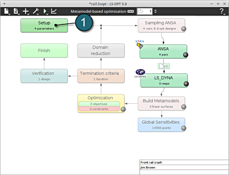
- Select the Setup box.
- A window Problem global setup shall open.
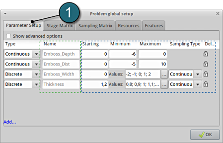
Define the Parameters.
- Select the Parameter Setup tab.
- The variables are already defined in the input file rail_DV.txt (shown below) .
# DESIGN VARIABLES
#-----------------------------------------------------------------------------------
# ID | DESIGN VARIABLE NAME | TYPE | RANGE| CURRENT VALUE|MIN VALUE-->MAX VALUE|STEP
#-----------------------------------------------------------------------------------
 1,  Emboss_Depth,  REAL,     BOUNDS,    0., -6., 0.
 2,  Emboss_Width,  REAL,     STEP,      0., -2., 2.,  1.
 3,  Emboss_Dist,  REAL,     BOUNDS,    0., -5., 10.
 4,  Thickness,  REAL,     LIST,    1.2,0.8,0.9,1.,1.1,1.2,1.4,1.7
#-----------------------------------------------------------------------------------
Stage Matrix
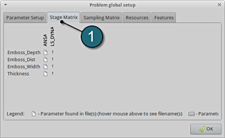
- Select the Stage Matrix tab.
- You find a matrix of parameters vs. stages, and symbols that visualize if parameters are found in input files. The names of the respective input files can be visualized by hovering the mouse on the respective file icon.
Sampling Matrix
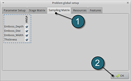
- Select the Sampling Matrix tab.
- If you don't want to use a parameter as variable for a respective sampling, the variables can be switched off here. The parameters are treated as constants then.
- Select the OK button to proceed.
Home Screen Process Flowchart
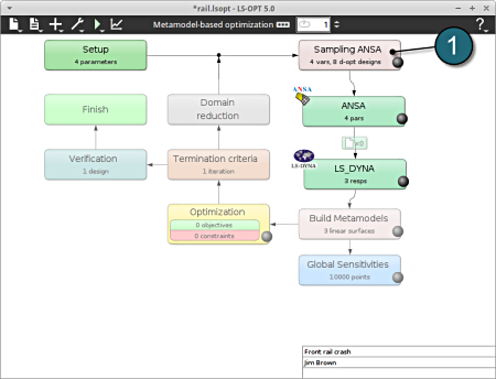
- Select the Sampling ANSA box.
A window Sampling ANSA shall open.
Define Metamodel Settings
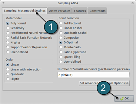
- Select the Sampling Metamodel Settings tab.
The default setup is kept unchanged at :
- For Metamodel : Polynomial.
- For Order : Linear.
- For Point Selection : D-Optimal.
- Select the OK button to proceed.
Build Metamodels
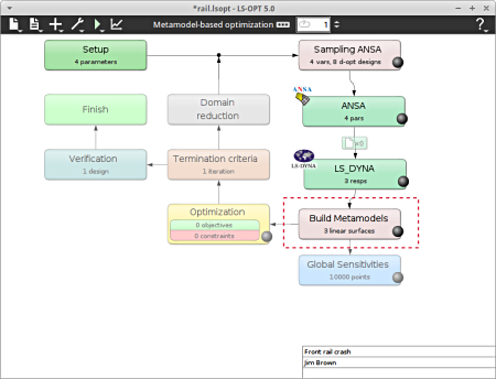
- To review the Metamodel properties for optimization, select the Build Metamodels box.
A window Sampling ANSA shall open which is the same as in the Sampling box.
Home Screen Process Flowchart
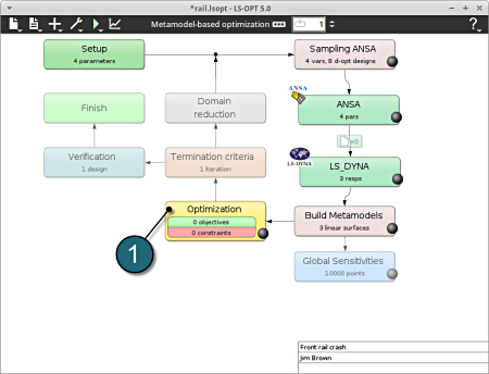
- Select the Optimization box.
A window Optimization shall open.
Add Objective
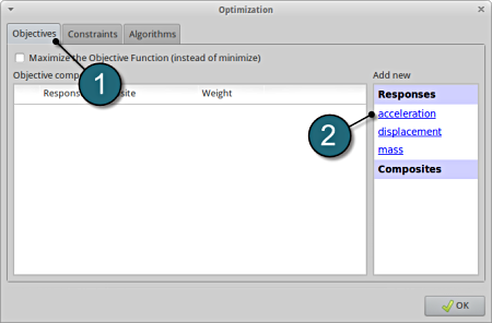
- Select the Objectives tab.
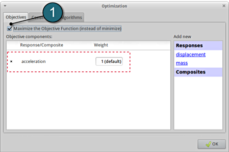
- From Responses select acceleration as the objective.
Define Objective
- Since the acceleration is negative, select the option Maximize the Objective Function (instead of minimize)
- For Weight leave the default 1. If you have several objective functions, you may assign weight to each one according to their importance.
Add Constraints.
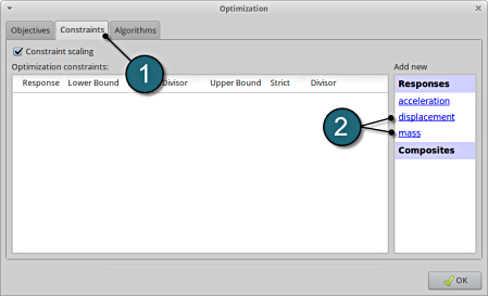
- Select the Constraints tab.
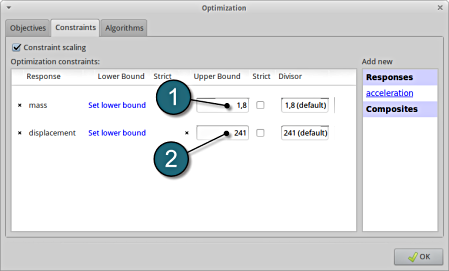
- From Responses select mass and displacement as the Optimization constraints.
Set bounds for Constraints.
- Select Set Upper Bound for mass at 1,8.
- Select Set Upper Bound for displacement at 241.
Optimization Algorithm.
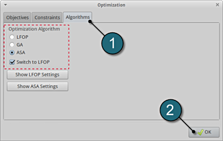
- Select the Algorithms tab. Here, the algorithm used for the optimization on the metamodel can be selected.
- Make sure that the radio button for Adaptive Simulated Annealing (ASA) is selected and Switch to LFOP is checked. These are the default settings.
- Select the OK button to proceed.
Home Screen Process Flowchart
-
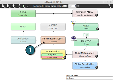
Select the Termination criteria icon.
A window Termination criteria shall open.
Define the Termination criteria
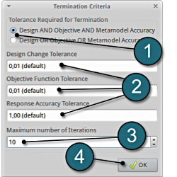
- Retail the (default) selection of the radio button on Design AND Objective AND Metamodel Accuracy for the choice of Tolerance Required for Termination.
- Several Tolerance parameters (Design, Objective, Response) are retained to their default values.
- Change the Maximum number of Iterations to 10.
- Push the OK button to proceed.
Run LS-Opt.
Baseline Run
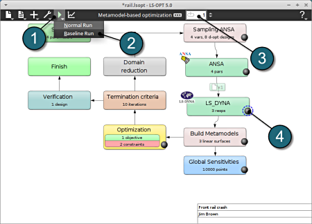
- Select the Run button from the Control Bar.
- Push Baseline Run for execution.
- Baseline Run: Helps to check the process for error free execution, which otherwise would cost unneceassry loss of computation time.
- The user can get information on the current iteration during execution.
- At every stage the user has an option to view the progress of the program execution by selecting the LED on the respective task box.
Normal Run
- In the similar way the user can execute a Normal Run.
Note: To understand the activity please refer to the example Crashworthiness Optimization.
After completion of the program execution the user can view the Results.
Home Screen Process Flowchart
- The results can be viewed by selecting the view button on the task bar. A seperate window of LS-OPT Viewer opens up.
LS-OPT Viewer
- Choose History under the category Optimization.
Input Variables
Select Variables → Emboss_Depth
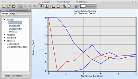
Fig. 1(a) shows:
- The optimization history of the variable Emboss_Depth.
- The development of the variable value of the optimum (red line)
- How the range of Emboss_Depth (set from -6 to 0 at the beginning) decreases after every iteration (blue lines).
- This variable is important (see Sensitivities) to reach the bounds of the constraint and minimize the objective and seems to be converged.
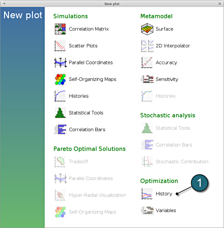
Fig. 1(a)
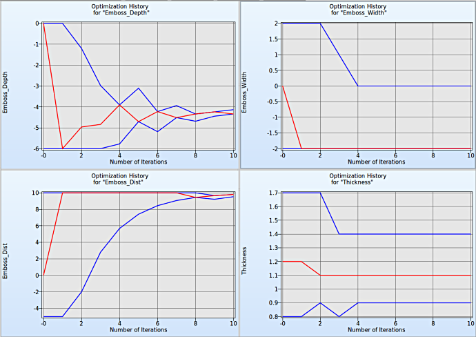
To compare multiple plots for covergence behaviour of the input variables, the user can select the split option at the task bar and select the other variables.
Fig. 1(b) Input variables convergence behaviour
It is evident from Fig. 1(b) that the input variables Emboss_Depth and Emboss_Dist have good convergence behaviour whereas Emboss_Width and Thickness do not tend to converge beyond a certain point even with additional iterations.
Constraints
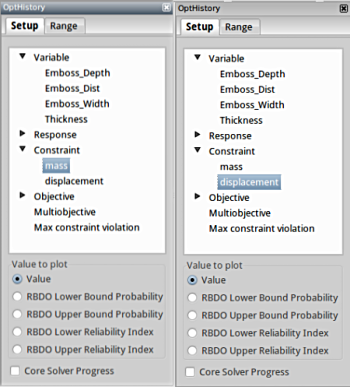
Select Constraints → mass
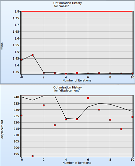
- Following similar steps, the user can view the Optimization history for the constraints of optimization, in this case for mass.
- To compare multiple plots for contraints, the user can select the split option at the task bar and select the other constraint.
Fig. 2 shows :
- The predicted result (black line) of the optimal constraints for every iteration.
- The computed result (red points) of the constraints for every iteration.
- The constraints upper bound (red line).
Fig. 2 Optimization History for Constraints
Objective
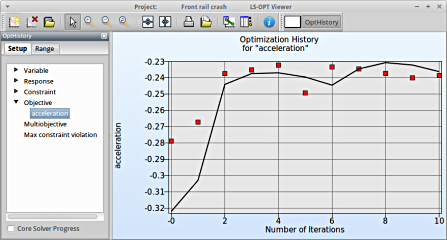
In the similar way the user can check the convergence of the main objective of the optimization.
Select Objective → acceleration
- The predicted result (black line) of the optimal objective acceleration for every iteration.
- The computed result (red points) of the optimal objective acceleration for every iteration.
- The convergence trend of the acceleration objective.
New Plot
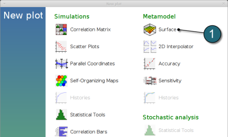
To view a new plot select the plot button on the task bar. A seperate window of LS-OPT Viewer opens up.
LS-OPT Viewer
- Select under Metamodel the item Surface.
- Slide to the last iteration (10).
- Select the Setup tab.
- Set the objective acceleration as the z-coordinate, the any two variables eg. Emboss_Depth and Emboss_Dist as the x-coordinate and y-coordinate, respectively.
- The other parameters are set to fixed values using the silders
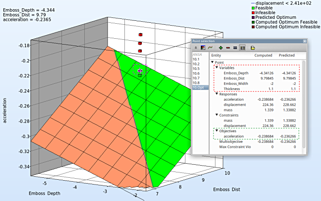
- Pick Constraints to visualize feasible and infeasible regions on the metamodel, respectively. The feasible region is drawn in green while the infeasible region is drawn in red.
- Choose Predicted value. A purple cross will appear somewhere on the surface. You can move it by changing the values of the variables. The predicted value for the selected parameter combination is displayed.
- Click Center on Opt. to locate the cross at the optimal point.
- Select the Points tab.
- For Iterations select Current.
- Pick Predicted Optimum and Computed Optimum.
- We rotate the plot with the mouse by pressing Ctrl at the meantime. The purple cube shows the predicted optimum value, while the green cube below denotes the computed optimum value, which is computed directly through the simulation model. Red points indicate that the point is infeasible.
- The user can view the values of all entities by selecting any point (or multiple points) in the plot ( in this case the predicted optimum ). A point selection window opens up showing the optimum values of the input variables (red outline) and the optimum objective value for acceleration (green outline).
New Plot
- To view a new plot select the plot button on the task bar. A seperate window of LS-OPT Viewer opens up.
LS-OPT Viewer
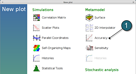
- Select under Metamodel the item Accuracy.
RMS Error and R2 Indicator
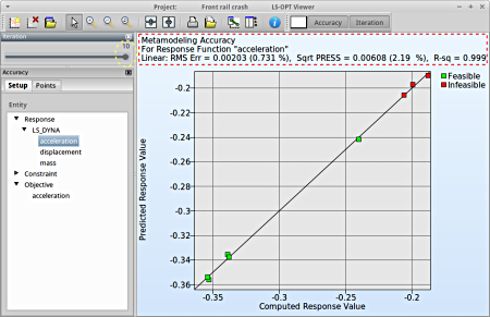
- From the left side of the window select Responses → acceleration.
- We can slide to observe the accuary of results at each iteration. In this case for Iteration 1.
- RMS Error, SPRESS and R2 (R-sq) can be found above the plot.
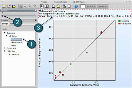
- At the last iteration (Iteration 10) we obtain a result with RMS Error = 0.002 (0.731%) and R2 = 0.999.
- A small RMS error and a coefficient of determination (R2) ~1 indicates good fit (see table below).
- A relatively low SPRESS (=2.19%) is observed which indicates a good prediction of the metamodel.
| RMS Error | R2 Indicator | |
| Small | ~1 | High variable detection: low noise, good fit. |
| Small | ~0 | Low noise/good fit, small gradient. |
| Large | ~1 | High variable detection with noise. |
| Large | ~0 | Lack of fit, perhaps accompanied by noise. Must shrink the move limits. |
We can find the development of RMS Error and R2 in History under Optimization.
New Plot
- To view a new plot select the plot button on the task bar. A seperate window of LS-OPT Viewer opens up.
LS-OPT Viewer
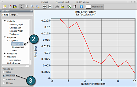
- Choose History under the category Optimization.
- Select from the left of the window Response → acceleration.
- Select RMS Error. We see that the RMS error is large at the 1st iteration and progressivly reduces till the 10th iteration.
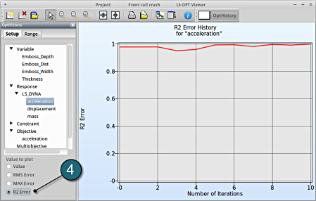
- Select R2 Error. The R2 error reaches its maximum near 1 across the iterations.
Which variable appears to be the most important?
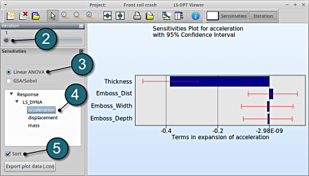
The significance of a variable for a response can be illustrated with ANOVA (analysis of variance) or GSA/Sobol (global sensitivity analysis), e.g for the response/objective acceleration you may find:
New Plot
- To view a new plot select the plot button on the task bar. A seperate window of LS-OPT Viewer opens up.
LS-OPT Viewer
ANOVA
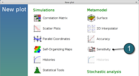
- Restart the LS-OPT Viewer and select under Metamodel the item Sensitivity
- We can slide to observe the sensitivity of results at each iteration. In this case for Iteration 1.
- Select Linear ANOVA in the new window.
- From Response select acceleration.
- Sort the variables according to their significance.
→ For the response acceleration the variable thickness is the most important, while the other variables are rather insignificant.
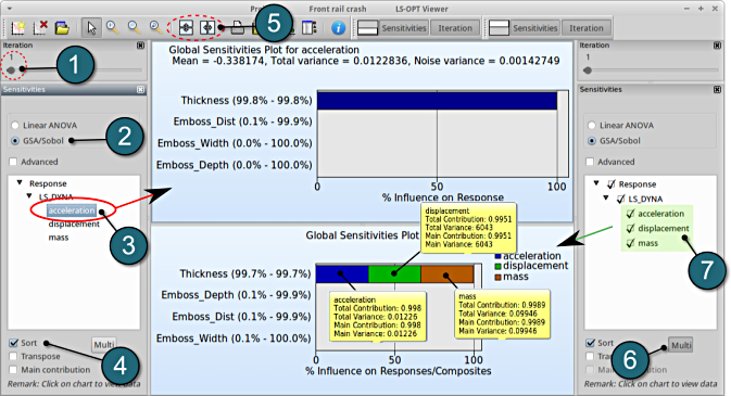
GSA/Sobol
- We can slide to observe the sensitivity of results at each iteration, in this case for Iteration 1
- Select GSA/Sobol in the new window.
- From Responses select acceleration.
- The user has the choice to Sort the plot by selecting the checkbox in the setup menu (default).
- To compare multiple plots for sensitivities of the input variables on the various responses, the user can select the split option at the task bar and repeat the previous steps.
- The viewer allows the user to select multiple responses for sensitivity analysis to get the influence of the variables on e.g. the whole problem or a load case using the following steps:
- Create a new plot area similar to step 5. Then select the option Multi.
- Select the necessary responses, in this case all the responses are selected .
- The plot describes the cumulative plot on a single graph w.r.t. the variables. This is only availabe for GSA, not for ANOVA, since GSA values are normalized.
The complete data set (input and command files) is available for download:
For Linux
For Windows

