Discrete optimization
Solving the optimization problem with a discrete variable.
Initial Steps
- Create a Working Directory in the desired location, e.g. Crash_Discrete.
- Extract all the files for the Discrete task from download section into the working directory.
- Load the srsm.lsopt file located in the Crash_Discrete by selecting from the Open other project. This is done in order to reduce repetative steps from the SRSM example.
- The main GUI window of LS-OPT opens.
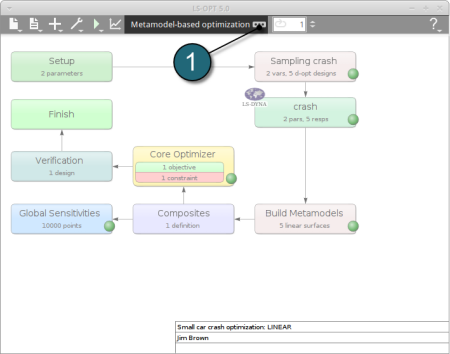
Home Screen Process Flowchart
- Select the Save as option from the taskbar. Save the file as discrete.lsopt.
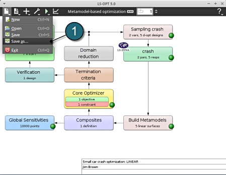
Home Screen Process Flowchart
-
Select the Task icon.
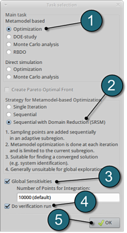
A window Task selection shall open.
Define the Main Task
- Select the radio button Optimization for the selection of the main objective for metamodel.
- The selection of the strategy for the metamodel is made to Sequential with Domain Reduction (SRSM).
- To study the various Global Sensitivities measures for the input parameter remember to select the radio .
- The user has a choice to Do verification run by selecting the option.
- Push the OK button to proceed.
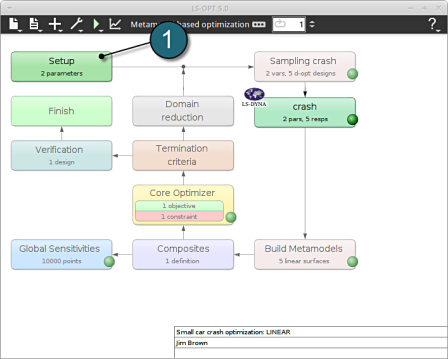
Home Screen Process Flowchart
- Select the Setup box.
A window Problem global setup shall open.
Define the Parameters.
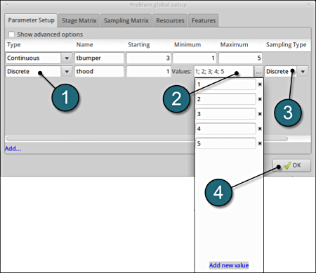
- Change Type of thood: switch the menu to Discrete.
-
Enter the Values ( 1;2;3;4;5 ) by selecting the option.
- Change the Sampling Type option to Discrete.
- Select OK to proceed.
Run LS-Opt.
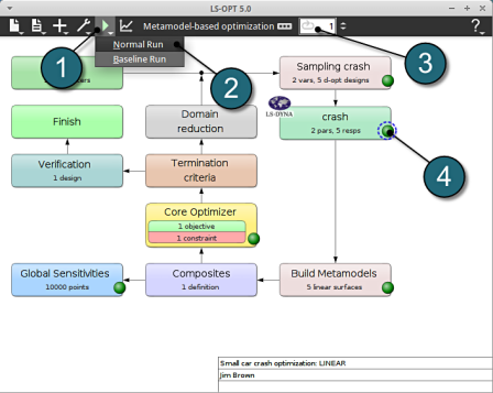
- Select the Run button from the Control Bar.
- Push Normal Run for execution.
- The user can get information on the status of the current iteration during execution.
- At every stage the user has an option to view the progress of the program execution by selecting the LED on the crash tab.
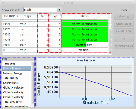
As seperate window Progress opens up.
Progress
- The progress bar gives information on the status and several other details of the optimization progress.
- Underneath the status, the user has the option to view various plots of the computed values during execution vs the simulation time.
After completion of the program execution the user can view the results.
View Log
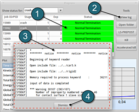
- Select the simulaiton point for which the log file is desired.
- Click on the View log button.
- A new window open containg the solver output, in this case the LS-DYNA output.
- Select the Dismiss button to close the window and proceed.
Home Screen Process Flowchart
- The results can be viewed by selecting the view button on the task bar. A seperate window of LS-OPT Viewer opens up.
LS-OPT Viewer
- Choose History under the category Optimization.
- We can choose from the left side the entities we want to observe.
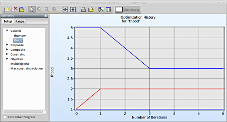
Select Variables → thood
Fig. 1(a) shows:
- The optimization history of the variable thood.
- The development of the optimal variable value (red line)
- How the range of thood (set from 1 to 5 at the beginning) decreases after every iteration (blue lines).
-
Observe the thood variable at every iterations takes discrete steps as assigned in the parameter setup.
- This variable is important (see Sensitivities) to reach the bounds of constraint and to minimize the objective and seems to be converged.
Fig. 1(a)
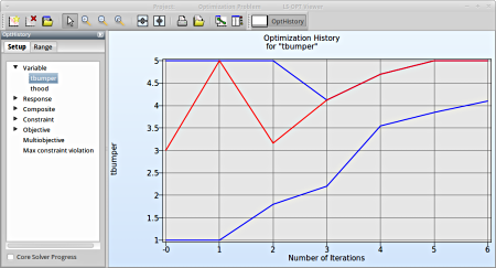
Select Variable → tbumper
Fig. 1(b) shows:
- The optimization history of the variable tbumper.
- The development of the optimal variable value (red line)
- This variable is rather insignificant (see Sensitivites) and therefore differs between the iteration without affecting the objective.
Fig. 1(b)
As you can see in the figure that the value of HIC doesn't change a lot between iteration 5 and 6. The tolerance for termination of 1% is reached and this will make LS-OPT stop the optimization process after 6 iterations although 10 iterations were specified in the Run panel.
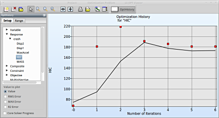
Select Response → crash → HIC
Fig. 2(a) shows:
- The predicted result (black line) of the optimal HIC response for every iteration.
- The computed result (red points) of the HIC response for every iteration.
- The convergence trend of the HIC response.
Fig. 2(a)
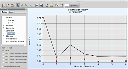
Select Constraint → Intrusions
Fig. 2(b) shows:
- The predicted result (black line) of the optimal Intrusion constraint for every iteration.
- The computed result (red points) of the Intrusion constraint for every iteration.
- The constraint upper bound is reached (red line).
We can plot the response surface of the metamodel we've built. For example, we want to see the response surface of HIC with respect to the variables thood and tbumper, do it as following:
New Plot
- To view a new plot select the plot botton on the task bar. A seperate window of LS-OPT Viewer opens up.
LS-OPT Viewer
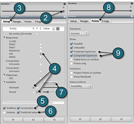
- Select under Metamodel the item Surface.
- Slide to the last iteration.
- Select the Setup tab.
- Set the response HIC as the z-coordinate, the variables tbumper and thood as the x-coordinate and y-coordinate, respectively.
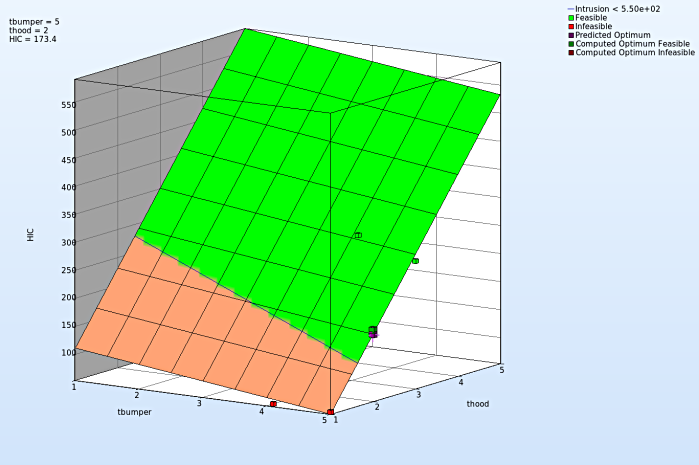
- Pick Constraints to show the constraints. The feasible region is drawn in green while the infeasible region is drawn in red.
- Choose Predicted value. A purple cross will appear somewhere on the surface. You can move it by changing the values of the variables tbumper and thood.
- Click Center on Opt. to locate the cross at the optimal point.
- Select the Points tab.
- Pick Predicted Optimum and Computed Optimum.
- We zoom up the plot and rotate it with mouse by pressing Ctrl at the meantime. The purple cube shows the predicted optimum value, while the green cube above denotes the computed optimum value, which is computed directly through the simulation model. Green indicates that the point is feasible.
Discrete variable - thood
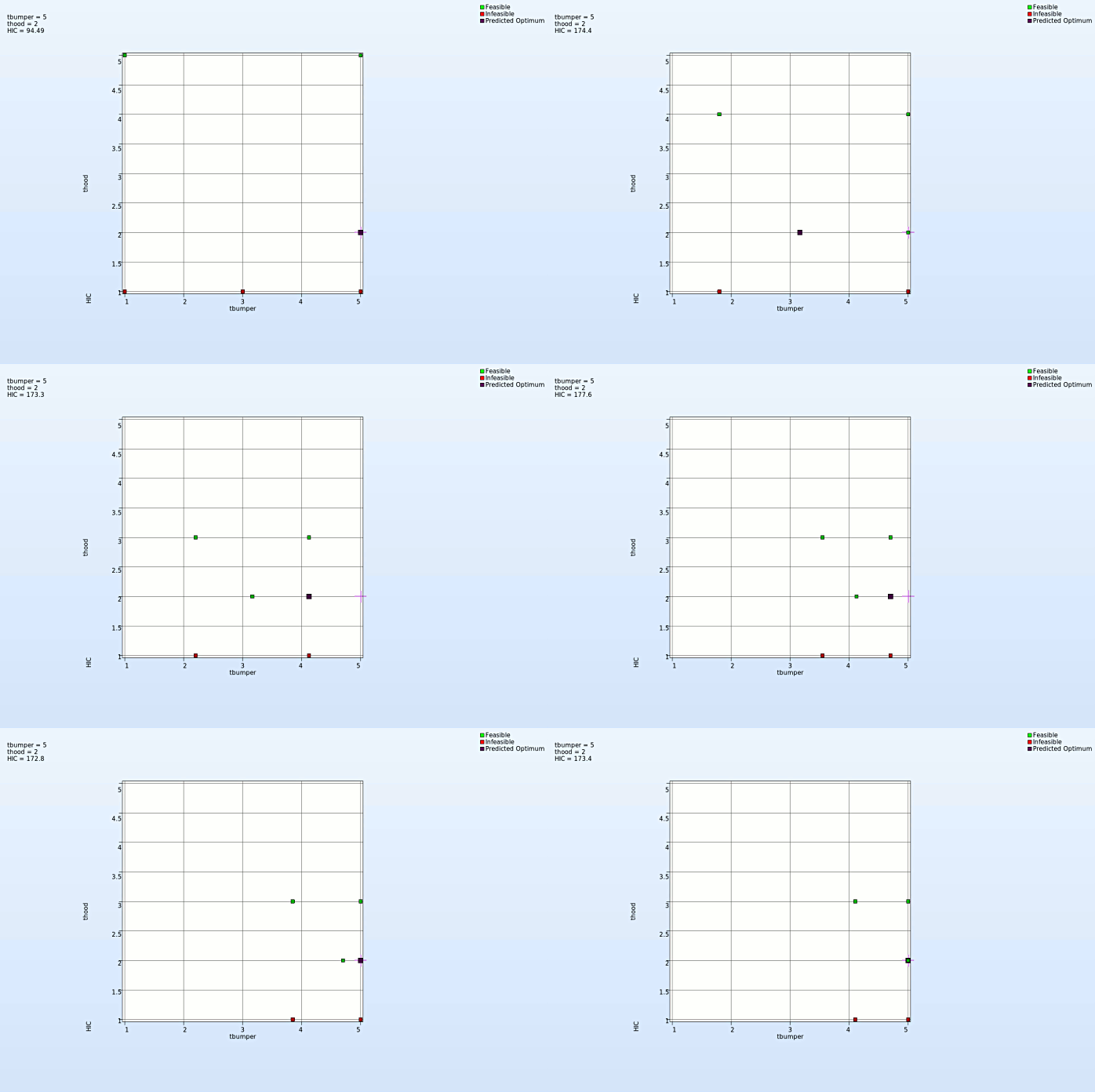
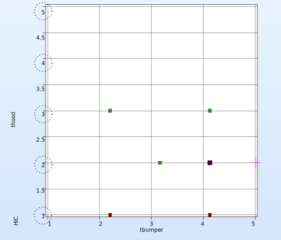
- At every step of iteration the varable thood takes discrete steps to reach the optimum. This is necessary because of manufaturing limitation.
- The discrete steps in the optimization process at every iteration is shown in the picture below.
New Plot
- To view a new plot select the plot botton on the task bar. A seperate window of LS-OPT Viewer opens up.
LS-OPT Viewer
- Select under Metamodel the item Accuracy.
RMS Error and R2 Indicator
- From the left side of the window select Responses → HIC.
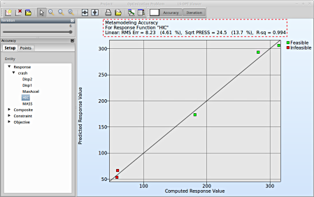
- RMS Error, SPRESS and R2 (R-sq) can be found above the plot.
- We can slide to observe the accuary of results at each iteration. In this case for Iteration 1.
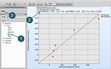
- At the last iteration (Iteration 6) we obtain a result with RMS Error = 8.23 (4.61%) and R2 = 0.994.
- A small RMS error and a coefficient of determination (R2) ~1 indicates good fit (see table below).
- The SPRESS value is average (=24.5%) indicating a moderate prediction of the metamodel fit.
| RMS Error | R2 Indicator | |
| Small | ~1 | High variable detection: low noise, good fit. |
| Small | ~0 | Low noise/good fit, small gradient. |
| Large | ~1 | High variable detection with noise. |
| Large | ~0 | Lack of fit, perhaps accompanied by noise. Must shrink the move limits. |
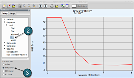
We can find the development of RMS Error and R2 in History under Optimization.
New Plot
- To view a new plot select the plot botton on the task bar. A seperate window of LS-OPT Viewer opens up.
LS-OPT Viewer
- Choose History under the category Optimization.
- Select from the left of the window Response → HIC
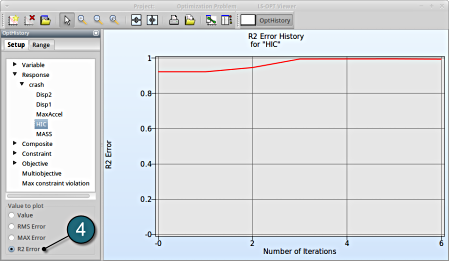
- Select RMS Error. We see that the RMS error is large at the 1st iteration and progressivly reduces till the 3rd iteration.
- Select R2 Error. The R2 error reaches its maximum near 1 at the 4th and remains till the 6th iteration.
The complete data set (input and command files) is available for download:
For Linux
For Windows


