Solution with LS-OPT
https://www.lsoptsupport.com/examples-4.0/optimization-example/solution-with-ls-opt
https://www.lsoptsupport.com/@@site-logo/LS-Opt-Support-Logo480x80.png
Solution with LS-OPT
Objective Function
- Select the Objective panel.
- Choose the Response Weight as objective
The created command file may look like this:
$$$$$$$$$$$$$$$$$$$$$$$$$$$$$$$$$$$$$$$$$$$$$$$$$$$$$$$
Command file "com"
$$$$$$$$$$$$$$$$$$$$$$$$$$$$$$$$$$$$$$$$$$$$$$$$$$$$$$$
$ Generated using LS-OPT Version 4.1
$
"Optimization Problem"
$
$ Created on Fri Nov 19 11:32:44 2010
solvers 1
responses 1
$
$ NO HISTORIES ARE DEFINED
$
$
$ DESIGN VARIABLES
$
variables 2
 Variable 'X' 0.
  Lower bound variable 'X' -1.
  Upper bound variable 'X' 3.
 Variable 'Y' 0.
  Lower bound variable 'Y' -1.
  Upper bound variable 'Y' 3.

$$$$$$$$$$$$$$$$$$$$$$$$$$$$$$$$
$      OPTIMIZATION METHOD
$$$$$$$$$$$$$$$$$$$$$$$$$$$$$$$$
$
Optimization Method SRSM

$$$$$$$$$$$$$$$$$$$$$$$$$$$$$$$$
$      SOLVER "1"
$$$$$$$$$$$$$$$$$$$$$$$$$$$$$$$$
$
$ DEFINITION OF SOLVER "1"
$
 solver own '1'
  solver command "perl"
  solver input file "/home/yu/optimierung/function"
$ ------ Pre-processor --------
$   NO PREPROCESSOR SPECIFIED
$ ------ Post-processor --------
$   NO POSTPROCESSOR SPECIFIED
$ ------ Metamodeling ---------
  solver order linear
  solver experiment design dopt
$ ------ Job information ------
  solver concurrent jobs 1
$
$ RESPONSES FOR SOLVER "1"
$
 response 'F' 1 0 "cat out.txt"

$
$ OBJECTIVE FUNCTIONS
$
 objectives 1
 objective 'F' 1
$
$ THERE ARE NO CONSTRAINTS!!!
$
 constraints 0
$
$ PARAMETERS FOR METAMODEL OPTIMIZATION
$
 Metamodel Optimization Strategy DOMAINREDUCTION
$
  iterate param design 0.01
  iterate param objective 0.01
  iterate param stoppingtype and
$
$ OPTIMIZATION ALGORITHM
$
 Optimization Algorithm hybrid simulated annealing
  Use GSA
$
$ JOB INFO
$
 iterate 10
STOP
Select a Strategy for Metamodel-based Optimization
Select the Strategy tab.
- Switch the radio button of the section “Strategy for Metamodel-based Optimization” to “Sequential with Domain Reduction (SRSM)” so that we can set the "Number of Iterations" later.
Define Solver and Input File
- Select the Solvers tab.
- For Solver Package Name select User-Defined because our example will not work with LS-DYNA but use Perl as the solver.
- For Command specify perl (since this is the solver)
- For Input File browse the file function.
- For Name of Analysis Case enter 1.
- Push the Add button.
Define the Variables
- Select the Variables tab.
- For Type of ”X” switch the combo box to Variable.
- Enter -1 for the Minimum of the variable.
- Enter 3 for the Maximum of the variable.
- For Type of “Y“switch the combo box to Variable.
- Enter -1 for the Minimum of the variable.
- Enter 3 for the Maximum of the variable.
Sampling Panel
- Select the Sampling Panel.
- Switch the radio button of the section “METAMODEL” to “Polynomial” and the radio button of the section “Order” to “Linear”. In “POINT SELECTION” use the default options “D-Optimal” and “Number of Simulation Points per Iteration per Case” = 5.
Responses Panel
- Select the Responses panel.
- Select USERDEFINED.
- We obtain the output of the response with the shell command cat out.txt. This file was written by our perl script. Note: Windows user may use the DOS command type instead of the shell command cat.
- For the Response Name we enter "F".
- Push the Add button to create the new response
Run the Optimization
- Select the Run panel.
- For Numer of iterations enter 10.
- Push the Run button to start the optimization. (Save the project as com in the same folder where you'd put the file function)
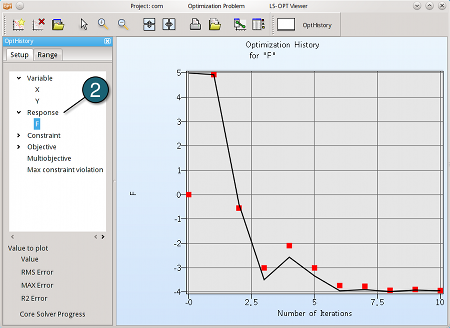
Optimization History For Response "F"
The Optimization History is a good tool to monitor the progress of our optimization. The view will be updated continuously after each iteration while the optimization is running.
Start the LS-OPT Viewer (Select the Viewer panel in the LS-OPT GUI) and
- Select History under subtitle "Optimization".
- A new window will appear, then select under "Setup" tab Response → F.
→ We can see, that with 3 iterations
there is still no convergence.
→ At the 6'th iteration we can see
that the response is getting close
to the optimal point.
→ After 10 iterations a good 
convergence can be observed.
We can conclude that perhaps
less than 10 iterations would
have sufficed to find the optimum.
The complete data set (input and command files) is available for download:
For Linux
For Windows
