Linear Sensitivity Analysis
In a first step, a linear sensitivity analysis is performed to identify the variables with high influence on the responses for each discipline. For both crash load cases 60 and for the NVH load cases 75 LS-DYNA simulations were performed. Since the number of variables is relatively high (27 for crash, 32 for stiffness/eigenvalues) a non-linear sensitivity analysis would require significantly more simulations.
https://www.lsoptsupport.com/examples-4.0/full-vehicle-mdo-example/linear-sensitivity-analysis
https://www.lsoptsupport.com/@@site-logo/LS-Opt-Support-Logo480x80.png
Linear Sensitivity Analysis
In a first step, a linear sensitivity analysis is performed to identify the variables with high influence on the responses for each discipline. For both crash load cases 60 and for the NVH load cases 75 LS-DYNA simulations were performed. Since the number of variables is relatively high (27 for crash, 32 for stiffness/eigenvalues) a non-linear sensitivity analysis would require significantly more simulations.
Define Solver and Input File
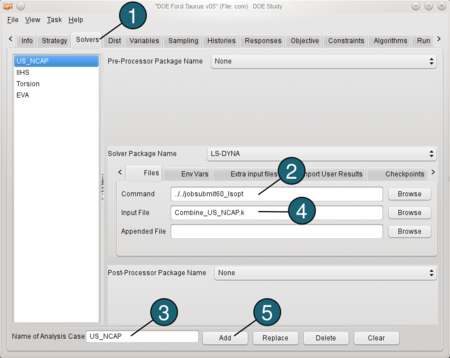
- Select the Solvers panel.
- For Command specify ../../jobsubmit60_lsopt (It is a script, that transmits the job to a cluster. This script can be different on your computer).
Make sure, that you specify an appropriate queuing system in the Run panel. - For the first load case enter a name for Name of Analysis Case, e.g. US_NCAP.
- Browse the Input File: Combine_US_NCAP.k.
- Push the Add button.
Repeat steps 3 - 5 for the rest of load cases, updating names and input files (see in the table below).
|
|
Load Case
|
Input File
|
| US_NCAP |
Combine_US_NCAP.k |
| IIHS |
Combine_IIHS.k |
| Torsion |
01_Taurus_Torsion__Master_v01_impl_linr_weg_param.key |
| EVA |
01_Taurus_EWA_Master_v03_param.key |
Define the Variables
- Select the Variables tab. The variables are
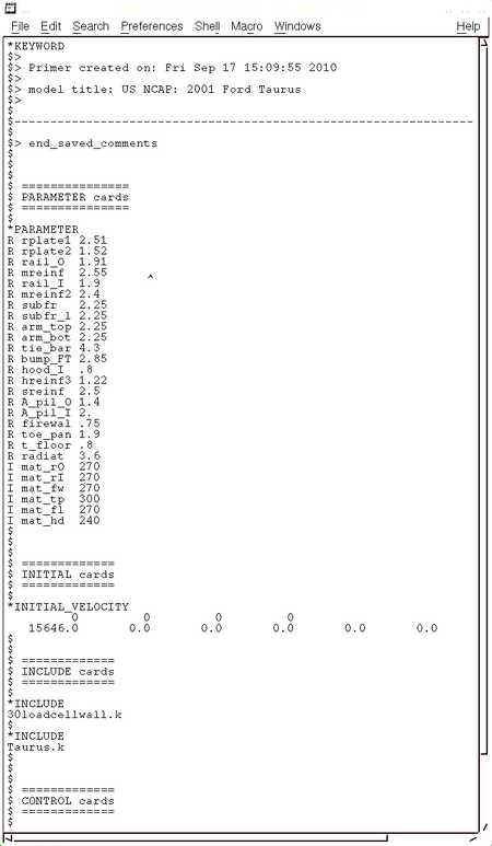
already defined in the input files Combine_US_NCAP.k, Combine_IIHS.k, 01_Taurus_Torsion_Master_v01_impl_linr
_kraft_param.key and 01_Taurus_EWA
_Master_v03_param.key using *PARAMETER (see the input file example for US_NCAP below). Therefore they cannot be deleted. This is indicated by the lock symbol on the left of the variable name. But you may change the initial value, if required.
On the right you can also see the solvers (disciplines) each variable is assigned to, e.g. mat_rO is assigned to US_NCAP and IIHS (local variable), whereas rplate1 is defined for all load cases (global variable). - The first six material variables are discrete variables defining different steel types. So for Type switch the menu to Discrete Var.
- Enter e.g. 270 300 340 370 410 480 800 for the list of allowable Values of the variable mat_rO. The value is the yield stress of the respective material.
- For Sampling Type switch to Discrete.
(For details see FAQs.) - For Type of remaining variables switch the menu to Variable.
- Enter 2 for the Minimum of the variable rplate1.
- Enter 3 for the Maximum of the variable rplate1.
Repeat steps 3 and 4 with the rest of discrete variables, updating the discrete values for each variable. Repeat steps 6 and 7 with the rest of variables, updating minimum and maximum for each variable. | 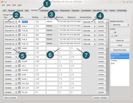
|
Choose the Sampling
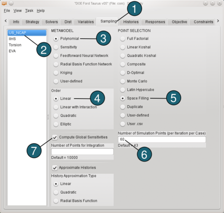
For the load case US_NCAP:- Select the Sampling tab.
- Select the load case US_NCAP.
- For METAMODEL select from the list Polynomial response surface.
- For approximation Order of the Polynomial model we take Linear.
(At this point, we took a linear polynomial metamodel, because the model is too large to be able to performe enought simulations to show nonlinearities. If possible, it's better to do more simulations and use e.g. Radial Basis Function Networks.) - Make sure that the Point Selection is set to Space Filling.
- Type 60 for Number of Simulation Points.
(approx. 2*number of variables recommanded for DOE) - Make sure that the Compute Global Sensitivities is selected for all load cases. It is necessary for the global sensitivity analysis - Sobol (see Results → Sensitivities).
| 
|
For the load case IIHS:Repeat steps 3 and 4. For Point Selection choose Duplicate and for Case US_NCAP, thus the simulation points are the same as for US_NCAP. |
For the load case Torsion:Repeat steps 3 - 5 and type 75 for the Number of Simulation Points. We take here a larger number because for the load case Torsion and EVA are more variables defined. |
For the load case EVA:Repeat steps 3 and 4. For Point Selection choose Duplicate and for Case Torsion, thus the simulation points are the same as for Torsion. |
Define the Histories
Histories are vectorial output entities of the simulations, e.g. displacement over time curves. Histories may be used to define scalar output entities, e.g. the maximal displacement.
Load case US_NCAP
Define x-acceleration of nodes: - Select the Histories tab.
- From the possible history types select: NODOUT.
- For Component select from the list Acceleration.
- For Direction select X Component.
- For Node ID enter 3740178.
(The acceleration of the left seat is measured by node 3740178.
To see the position of the node click on the ID-number.) - For Filtering choose SAE Filter.
- Enter 60.0 for Frequency.
- For Case switch to US_NCAP.
- For History Name enter accel_left_seat.
- Push the Add button.
For the rest of the Acceleration-Histories ( e.g. accel_right_seat, accel_engine_top, accel_engine_bottom, accel_B_pillar_r, accel_B_pillar_l ) repeat the steps 2 to 10, updating only the Node IDs and Names. | 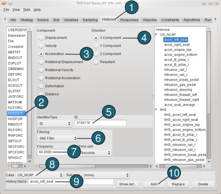
|
Define intrusion: - From the possible history types select: NODOUT.
- For Component select from the list Deformation.
- For Direction select X Component.
- For Coordinate System select Local.
- For Identifier Type switch to ID.
- For Local x-axis from enter 2362340 to 2352390, 3rd node ID 2214602.
- For Measured Node ID enter 2057404.
(To see the position of the node click on the ID-number.) - For Reference Node ID enter 2362340.
- For Filtering choose None.
- For Case switch to US_NCAP.
- For History Name enter intrusion_rail_l.
- Push the Add button.
For the rest of the Intrusion-Histories ( e.g. intrusion_rail_r, intrusion_break_pedal, intrusion_gas_pedal, intrusion_steering, intrusion_firewall_left, intrusion_firewall_right) repeat the steps 1 to 12, updating only the Measured Node IDs and Names. | 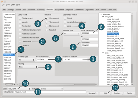 |
Define an Expression: Now we would like to calculate the average accelaration of a seat. Therefore we use the predefined histories accel_left_seat and accel_right_seat. - From the possible history types select: Expression.
- In the input field for an algebraic expression enter (accel_left_seat+accel_right_seat)/2.
- For Case switch to US_NCAP.
- For History Name enter accel_seat_average.
- Push the Add button.
Define the same histories for the load case IIHS, that you defined for the load case US_NCAP. | 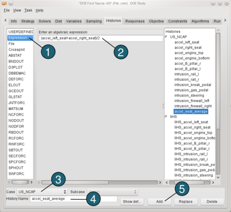 |
Load case Torsion
Define Displacement: - From the possible history types select: RBDOUT.
- For Rigid Body ID enter 2000804.
- For Component select from the list Displacement.
- For Direction select Z Component.
- For Case switch to Torsion.
- For History Name enter z_displ_2000804.
- Push the Add button.
Repeat steps 1 to 7 to define other displacements ( e.g. z_displ_2000805, y_displ_2000804, y_displ_2000805), updating the IDs, Directions and Names. | 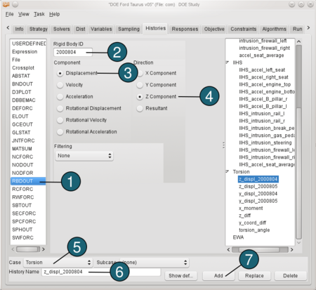 |
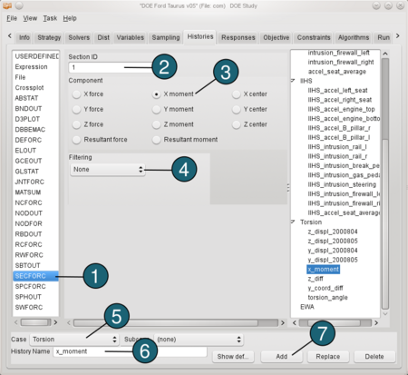
Define X-Moment: - From the possible history types select: SECFORC.
- For Section ID enter 1.
- For Component select from the list X moment.
- For Filtering choose None.
- For Case switch to Torsion.
- For History Name enter x_monent.
- Push the Add button.
|  |
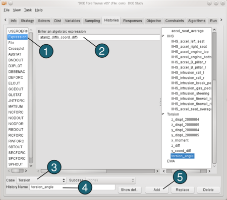
Define the torsion angle: We need to define two expressions before calculating torsion angle. The first one is the difference between the displacements in z direction we defined above (z_diff = z_displ_2000804 - z_displ_2000805). And the second one ist the difference between the coordinates of the displacements in y direction ( y_coord_diff = y_displ_2000804 - y_displ_2000805+1122.4566) The value 1122.4566 is the initial distance between the y coordinates. Now we can define the torsion angle: - From the possible history types select: Expression.
- In the input field for an algebraic expression enter atan(z_diff/y_coord_diff).
- For Case switch to Torsion.
- For History Name enter torsion_angle.
- Push the Add button.
|  |
Define the Responses
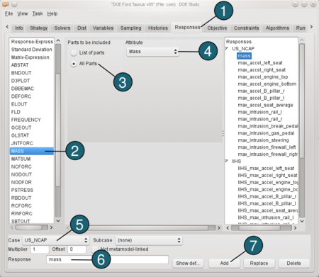
Define mass: - Select the Responses tab.
- From the possible response types select: MASS.
- For Parts to be included select: All Parts.
- For Attribute choose Mass.
- For Case switch to US_NCAP.
- For Response Name enter mass.
- Push the Add button.
|  |
Define maximum acceleration: - From the possible response types select: Response-Expression.
- For algebraic expression enter: -Min("accel_left_seat(t)").
(To define the expressions we can use here histories, that we defined in the Histories tab.)
Because the x-axis is defined in opposite direction of motion, we have to define the expressions for maximum as "-minimum". - For Case switch to US_NCAP.
- For Response Name enter max_accel_left_seat.
- Push the Add button.
For the rest of the maximum acceleration-responses ( e.g. max_accel_right_seat, max_accel_engine_top, max_accel_engine_bottom, max_accel_B_pillar_r, max_accel_B_pillar_l ) repeat the steps 1 to 5, updating the algebraic expressions and Names. The same applies to responses for maximum intrusion. | 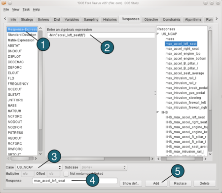
|
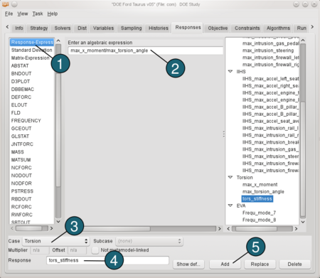
Define torsional stiffness: Before defining torsional stiffness we have to define two other response-expressions. These are the maximum x-moment (max_x_moment = Max("x_moment(t)") ) and the maximum torsion angle ( max_torsion_angle = Max("torsion_angle(t)") ). - From the possible response types select: Response-Expression.
- For algebraic expression enter: max_x_moment/max_torsion_angle.
- For Case switch to Torsion.
- For Response Name enter tors_stiffness.
- Push the Add button.
|  |
Define frequency mode 7: - From the possible response types select: FREQUENCY.
- For Baseline Mode Number type 7.
- For Modal Output Option select Frequency of Mode.
- For Case switch to EVA.
- For Response Name enter Frequ_mode_7.
- Push the Add button.
Repeat steps 1 to 6 for frequency mode 8. | 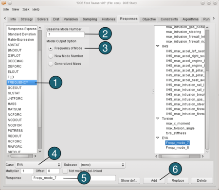 |
Constraints
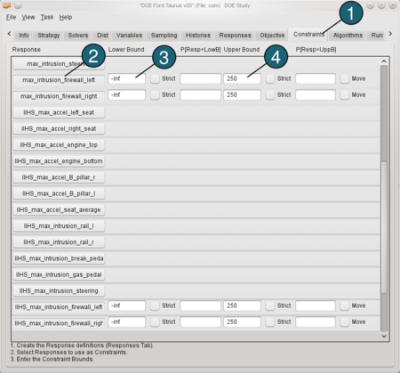
- Select the Constraints tab.
- From Response select max_intrusion_firewall_left, max_intrusion_firewall_right, IIHS_max_intrusion_firewall_left and IIHS_max_intrusion_firewall_right as constraints.
- For Lower Bound accept the default -inf.
- for Upper Bound enter 250.
|  |
Run LS-OPT
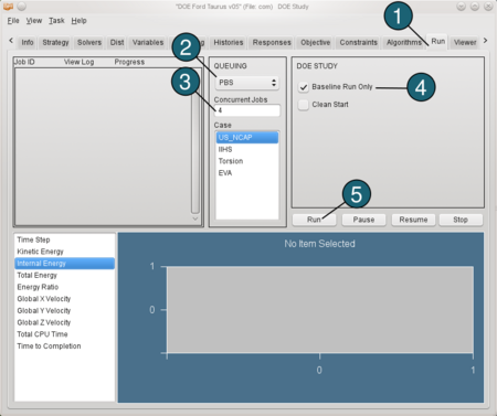
- Select the Run tab.
- Select a Queuing system.
Make sure, that you specified a script for solver command in the Solvers panel.
(For Details see the LS-OPT User's Manual chapter 9.12 Remote job scheduling.) - Type a number of Concurrent Jobs for each load case.
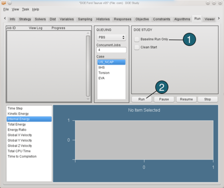
- Select Baseline Run Only.
(This feature provides the user with an option to run a single design, sampled at the initial values specified in the variables panel. This option facilitates a verification of the design problems.) - Push the Run button. (Save the project e.g. as com.)
| 
|
- If there are no problems after the baseline run, deselect the Baseline Run Only.
- Push the Run button.
|  |
Results of the simulated points for the selected iterations appear as dots on the scatter plots. This feature allows the three-dimensional plotting of any three entities. A forth dimension may be visualised using the color of the points. 2D plots can be obtained by selecting No entity for the z axis.
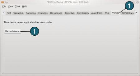
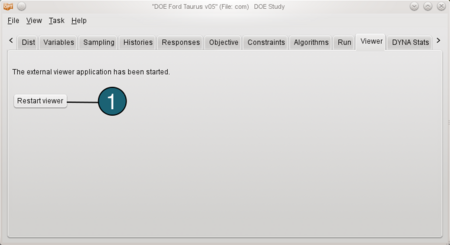
LS-OPT Viewer - Select the Viewer tab. The New plot window appear. Or restart the LS-OPT Viewer by clicking on the Restart viewer button.
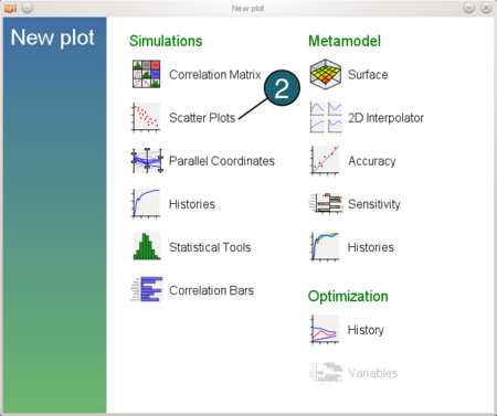
- Choose Scatter Plots as Type of Plot.
| 
|
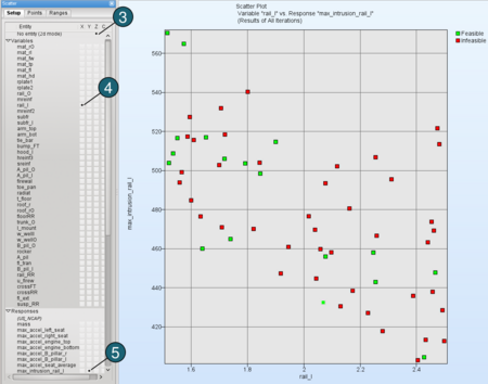
Variable "rail_l" vs. Response "max_intrusion_rail_l":- For the Z-axis select No entity to switch to the 2d mode.
- For the X-axis select the Variable rail_l.
- For the Y-axis select the Response max_intrusion_rail_l.
Feasible points are shown in green, infeasible points in red. The Figure shows the correlation between a variable and a response.
We could conclude: the bigger the thickness of the variable rail_l (see highlighted in red in the figure below), the smaller is the maximal intrusion of the response max_intrusion_rail_l. The remaining dimensions, that could also have influence on the response, are projected into the plot. 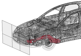
| 
|
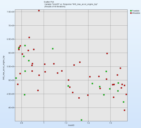
Variable "hreinf3" vs. Response "IIHS_max_accel_engine_top":
For the X-axis select the Variable hreinf3 and for Y-axis select IIHS_max_accel_engine_top. 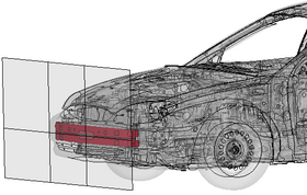
|  |
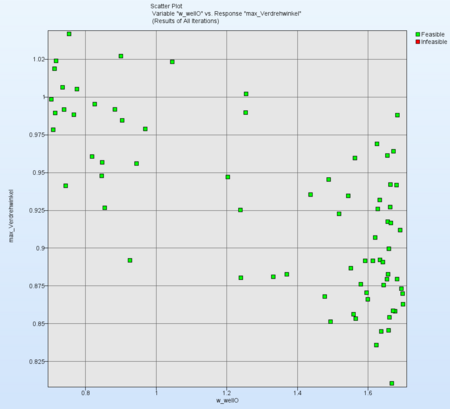
Variable "w_wellO" vs. Response "max_torsion_angle":For the X-axis select the Variable w_wellO and for Y-axis select max_torsion_angle. Obviously we can say: the bigger the thickness of the variable w_wellO (see highlighted in red in the figure below), the smaller is the maximal torsion angle. 
|  |
Variable "w_wellO" vs. Response "torsional_stiffness":For the X-axis select the Variable w_wellO and for Y-axis select tors_stiffness. We defined torsional stiffness as x-moment / torsion angle. As expected the scatter plot shows: the thicker the w_wellO, the smaller the maximal torsion angle (scatter plot above), the greater is the torsional stiffness. | 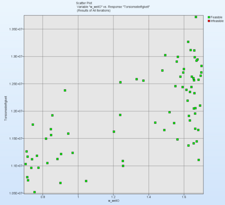 |
This plot visualizes history curves based on time data or crossplots obtained from simulations.
- Restart the LS-OPT Viewer either in the LS-OPTui by clicking on the Restart viewer button or click on new plot icon on the menu bar .
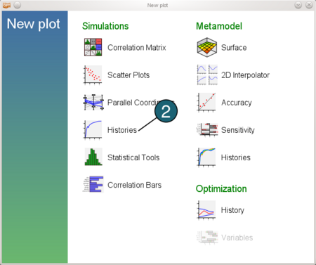
- Select under Simulations the item Histories.
| 

|
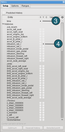
- As x-coordinate select time.
- Choose intrusion_rail_l as y-coordinate.
- Set the variables rail_l as c-coordinate.
(C-coordinate affects the color of each curve dependend on the value of the c-coordinate.)
|  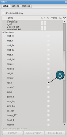 |
→ History curves of 60 simulations for intrusion_rail_l. The value of the variable rail_l determines the color of each curve.
There you can see, that the variable rail_l has a considerable influence on the response max_intrusion_rail_l. | 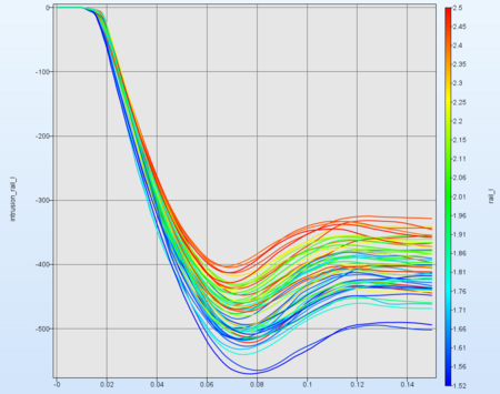 |
Choose now accel_seat_average as y-coordinate and leave the variable rail_l as c-coordinate. →The chaotic behaviour does not mean inevitable, that the variable does not have an influence on the response. It could be, that the influence of other variables leads to this behaviour. | 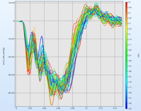 |
Two- or three-dimensional cross-sections of the metamodel surfaces and simulation points can be plotted and viewed from arbitrary angles.
Metamodel- Restart the LS-OPT Viewer either in the LS-OPTui by clicking on the Restart viewer button or click on new plot icon on the menu bar .
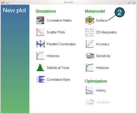
- Select under Metamodel the item Surface.
| 

|
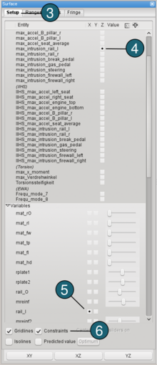
Set up the panels- Select the Setup panel.
- Choose max_intrusion_rail_l as z-coordinate.
- Set the variables rail_l and arm_top as x- and y-coordinate, respectively.
(The sliders allow changing the variable values for unselected variables (variables not plotted). The slider for the active variables can be activated by selecting the “Predicted Value” option, a purple cross is displayed on the metamodel showing the values for the selection.) - Select Constraints.
(Constraints are displayed on the surface.
Feasible regions are in green, the shade of red shows the degree of infeasibility (number of violated constraints), the colored
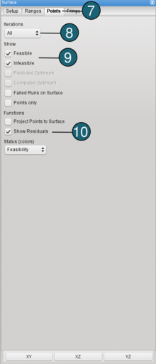
line show the location where the constraints are exactly met.) - Go to the Points panel.
- Turn Iterations to All.
- Show all the feasible and infeasible points.
- Select Show Residuals.
(Shows the deviation between the metamodel and predicted values as black vertical line.)
|   |
→The residuals are mainly small, thus you can say this is a well approximated metamodel.
Note the legend describing violated constraints on the top right. | 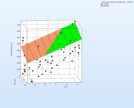 |
Select now for response max_intrusion_steering and for variables rail_l and A_pil_l.
→In comparison with the figure above the metamodel is not so well approximated. Almost all residuals are large. | 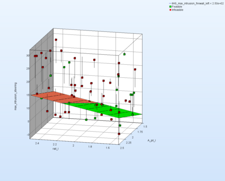 |
Which variable appears to be the most important?
The significance of a variable for a response can be illustrated with ANOVA (analysis of variance) or GSA/Sobol (global sensitivity ananlysis). Note that also GSA/Sobol illutstrates only the linear influence here, because we use a linear metamodel.
- Restart the LS-OPT Viewer either in the LS-OPTui by clicking on the Restart viewer button or click on new plot icon on the menu bar .
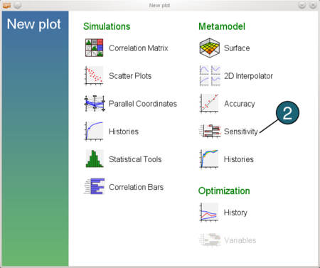
- Select under Metamodel the item Sensitivity.
| 

|
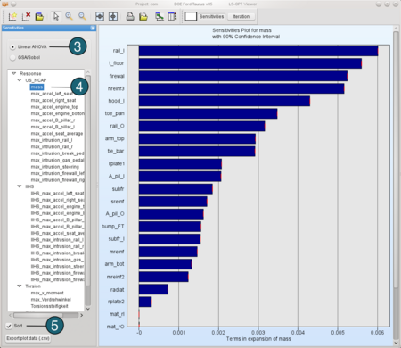
ANOVA- Select Linear ANOVA in the new window.
- From Response, e.g. for the load case US_NCAP, select mass.
(The influence of different variables on response mass is shown in the Figure below.) - Sort the variables according to their significance for mass.
→ For the response mass the variables rail_l and t_floor are the most important variables. (They are highlighted in red and blue in the figure below .) In contrast the variables mat_rl and mat_rO are insignificant. 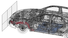
| 
|
The influence of different variables on response max_intrusion_rail_l: From Response select max_intrusion_rail_l for the load case US_NCAP, to see therefor the belonging diagramm. → rail_l and mat_rl are the most important variables. | 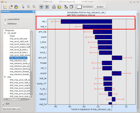
|
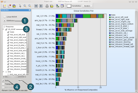
GSA/Sobol - Select the GSA/Sobol.
- Select Multi. (This option allows to select multiple responses.)
- From Response select US_NCAP.
(The influence of different variables on case US_NCAP is shown in the Figure.) - Sort the variables according to their significance for US_NCAP.
|  |
Select now from Response IIHS to see the influence of variables on this load case. | 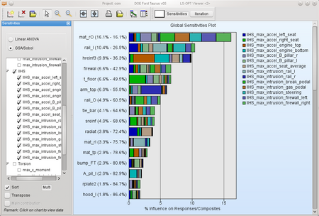 |
Sobol - Diagram for load case Torsion: | 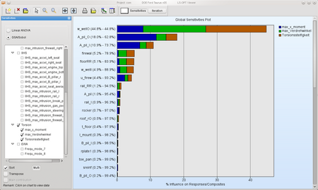 |
Sobol - Diagram for load case EVA: | 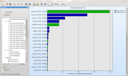 |
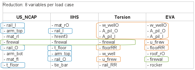
This information may be used to reduce the set of variables for each load case and e.g. perform an optimization afterwards. Here, 8 most important variables are selected for each load case. The colors in the table below visualize the common variables of the load cases. Obviously the variable firewal is important for all four load cases.
The command file is available for download:
For Linux
